FMMS: The Fused Matmul-Sample Kernel

TL;DR

I present FMMS, a Triton kernel to do fast and exact LLM sampling. It fuses the LM head matmul with token sampling, minimizing memory traffic in the memory-bound decoding regime. In kernel microbenchmarks across 4 datacenter GPUs (H100, H200, B200, B300), it is up to 1.25x faster than the fastest FlashInfer sampling kernel and up to 1.5x faster than PyTorch compiled sampling. Integrated into vLLM on B200, it reduces end-to-end TPOT across four models: up to 19% on Qwen3-1.7B, 7% on Qwen3-8B, 2% on Qwen3-32B, and 5% on gpt-oss-120b, with no accuracy loss.

The code is available on GitHub: github.com/tomasruizt/fused-mm-sample. The algorithm is explained in Section 3 and Section 7, kernel microbenchmarks are in Section 4, and end-to-end benchmarks on vLLM are in Section 5.

The Problem: GMEM Traffic

Every LLM decode step runs the same pipeline: multiply hidden states by the LM head weights to produce logits, normalize via softmax, then sample a token. The logits tensor has shape \([N, V]\), where \(V\) is the vocabulary size (up to 256K) and \(N\) is the batch size. In the standard approach, this entire tensor is written to GMEM and then read back for sampling. This round-trip is pure waste when the operation is memory-bound, which is the common case during decode (\(N \leq 64\)).

def sample(
    weights: torch.Tensor,       # [V, d]
    hidden_states: torch.Tensor, # [N, d]
):
    logits = hidden_states @ weights.T  # [N, V]
    probs = logits.softmax(dim=-1)      # [N, V]
    samples = torch.multinomial(probs, num_samples=1)
    return samples  # [N, 1]

Existing libraries assume the logits are already materialized: FlashInfer’s (Ye et al. 2025) sampling kernels take logits or probs as input, and Liger Kernel (Hsu et al. 2025) targets training rather than inference. Can the matmul and sampling be fused into a single kernel that never writes logits to GMEM?

The Solution: Fusion

FMMS (Fused Matrix Multiplication & Sampling) computes the matmul and samples in one kernel, without writing the full logits tensor to GMEM. Figure 1 contrasts the two approaches.

Figure 1: W is the LM head weight matrix, H is the hidden states for sampling. PyTorch materializes the full [N, V] logits in global memory (GMEM). FMMS keeps logits in shared memory (SHMEM) and writes only one scalar per tile. Red arrows are loads/stores to GMEM, green arrows stay in SHMEM.

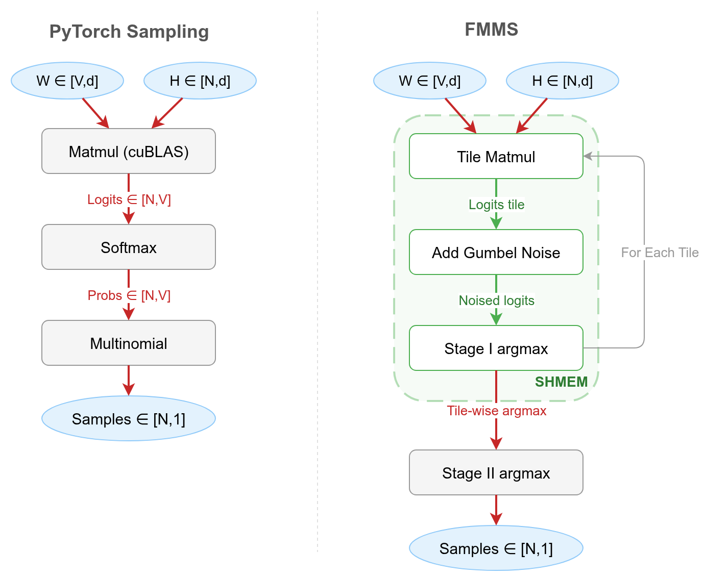
The trick is the Gumbel-max reparameterization (Huijben et al. 2021), which replaces softmax + multinomial with a single argmax over noised logits:

\[ \text{sample} = \text{argmax}_i \left( \frac{\ell_i}{\tau} + G_i \right) \sim \text{Categorical}(\text{softmax}(\ell / \tau)) \]

where \(G_i \sim \text{Gumbel}(0, 1)\) are i.i.d. noise variables, \(\ell_i\) are the logits, and \(\tau\) is the temperature parameter. The crucial property is that argmax decomposes over tiles. This works because the maximum of sub-maxima equals the global maximum, so each tile can independently find its local winner and a cheap reduction over tile-local winners produces the final sample. The kernel computes logits tile by tile, finds each tile’s winner, and discards the rest. This requires implementing the matmul in Triton rather than calling cuBLAS, because cuBLAS is a closed-box library call and fusion needs custom logic (noise generation, argmax) injected into the matmul’s inner loop.

Concretely, the kernel has two stages. In stage 1, a 2D grid of Triton programs tiled over (vocabulary, batch) each computes its logit block via matmul, adds Gumbel noise, finds the tile-local argmax, and writes only two scalars to GMEM: the maximum noised logit value and the corresponding vocabulary index. In stage 2, a cheap host-side reduction over these tile-local maxima picks the global winner per batch row. The full algorithm details come later in this post; the next section shows the benchmark results first.

Kernel Microbenchmarks

The LM head is a dense [V, d] matrix in every model, including MoE architectures (MoE only replaces the FFN layers, not the LM head). MoE models have surprisingly small hidden dimensions relative to their parameter count because the extra parameters live in expert FFN layers, not the LM head. I benchmark two workload sizes based on this analysis of LM head configurations across 25+ models:

• Small (V=151,936, d=4,096): Qwen3-8B, and notably Qwen3-235B MoE (which has d=4,096 despite 235B total parameters).
• Large (V=128,256, d=8,192): Llama 3 70B, DeepSeek V3 (d=7,168).

Baselines

Both FlashInfer kernels require the full logits, so their runtimes include the matmul that computes the logits. This is a fair comparison because FMMS also computes a matmul, the full logits tensor is just not written to GMEM.

1. FlashInfer top_k_top_p_sampling_from_logits: A dual-pivot rejection sampling kernel used in vLLM for top-k/top-p sampling.
2. FlashInfer sampling_from_logits: FlashInfer’s fastest sampling kernel. It also uses the Gumbel-max trick internally, but operates on pre-materialized logits.
3. PyTorch Compiled: torch compiled matmul + softmax + torch.multinomial.

All baselines are torch compiled, so the matmul dispatches to cuBLAS.

GPUs

Since FMMS saves memory bandwidth, its advantage depends on how memory-bound the workload is. I benchmark across four modern datacenter GPUs:

GPU	HBM Bandwidth (GB/s)	Peak BF16 (TFLOP/s)	Ops:Byte Ratio
B300	8,000	2,250	281
B200	8,000	2,250	281
H200	4,800	989	206
H100	3,350	989	295

The ops:byte ratio (peak compute / peak bandwidth) determines the crossover point where the matmul transitions from memory-bound to compute-bound. All experiments are reproducible. The GitHub README has setup instructions and make targets for all benchmarks and tests.

Scaling Behavior

Figure 2 shows execution time (left) and throughput in samples/ms (right) across batch sizes. All methods have nearly flat latency from N=1 to 32 (memory-bound: runtime is dominated by loading the weight matrix). Beyond N=64, latency rises as the matmul becomes compute-bound. FMMS (red) is the fastest method in the flat region, where fusion eliminates the extra GMEM round-trip for logits. At larger batch sizes, the baselines catch up as the matmul approaches the compute-bound regime and cuBLAS efficiency matters more.

Small

B300

Figure 2: Batch scaling on B300 (V=151,936, d=4,096).

B200

Batch scaling on B200.

H200

Batch scaling on H200.

H100

Batch scaling on H100.

Large

B300

Batch scaling on B300 (V=128,256, d=8,192).

B200

Batch scaling on B200.

H200

Batch scaling on H200.

H100

Batch scaling on H100.

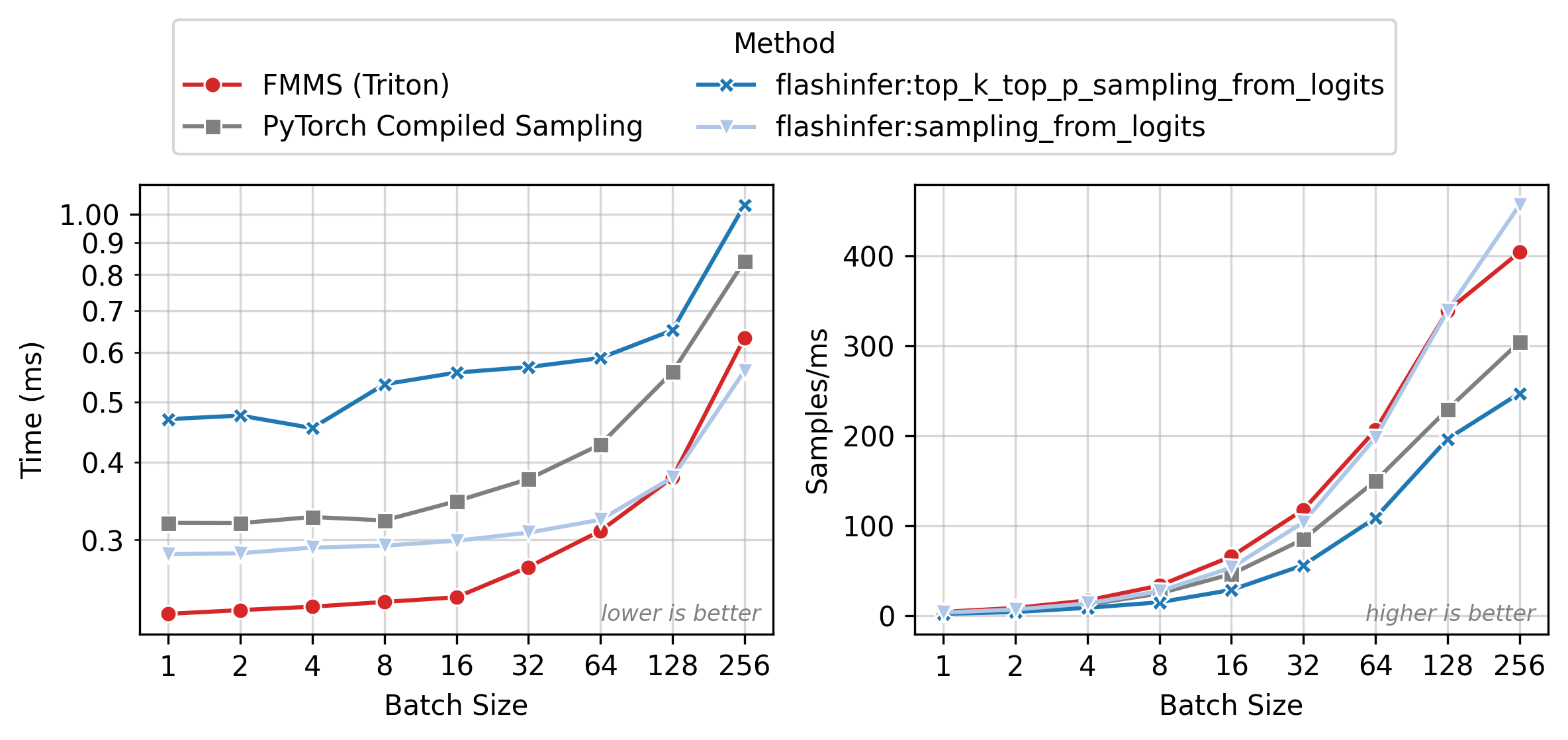
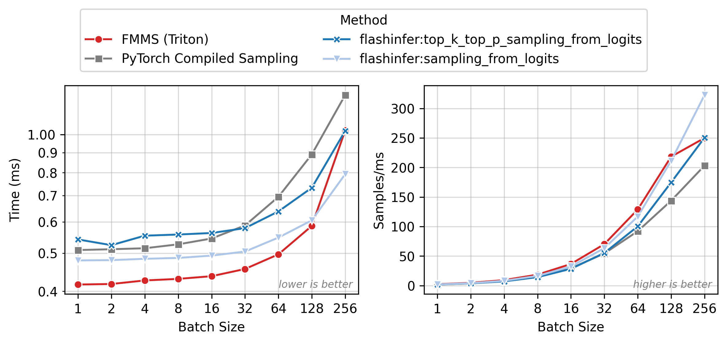
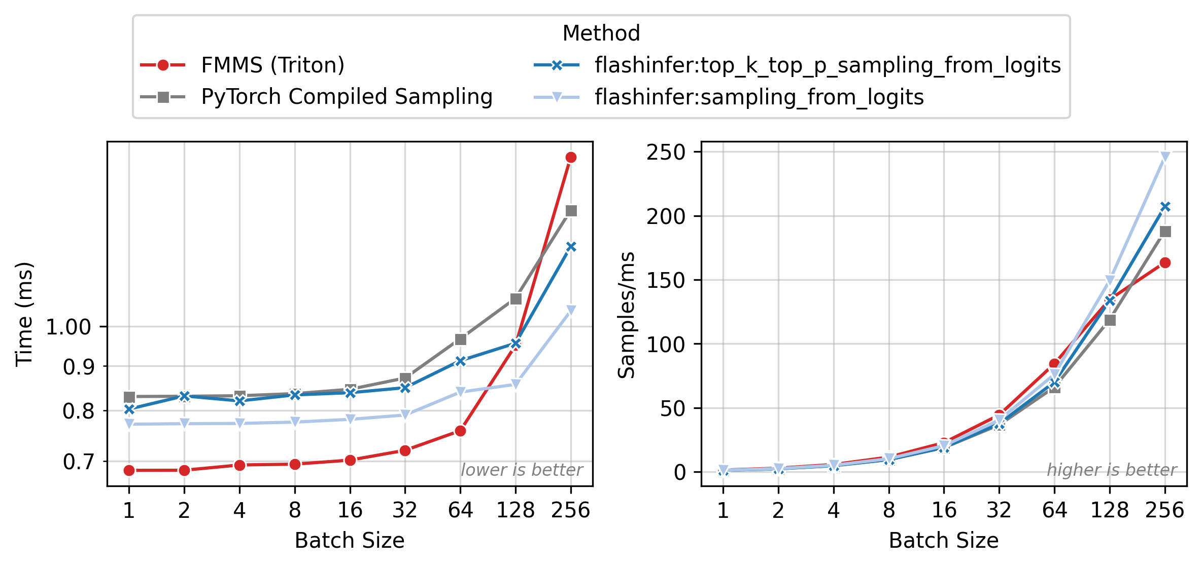
All benchmarks: PyTorch 2.10.0, CUDA 13.0, run on Modal. Data as of 2026-02-11.

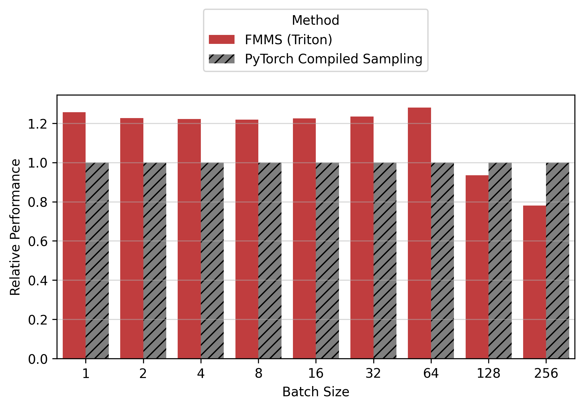
Relative Performance Across GPUs

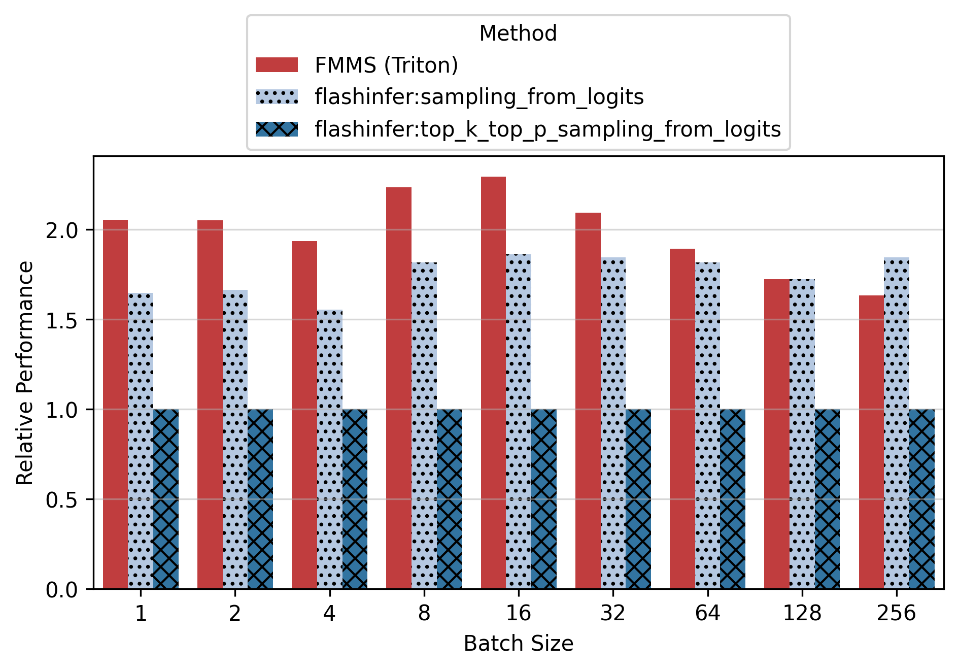
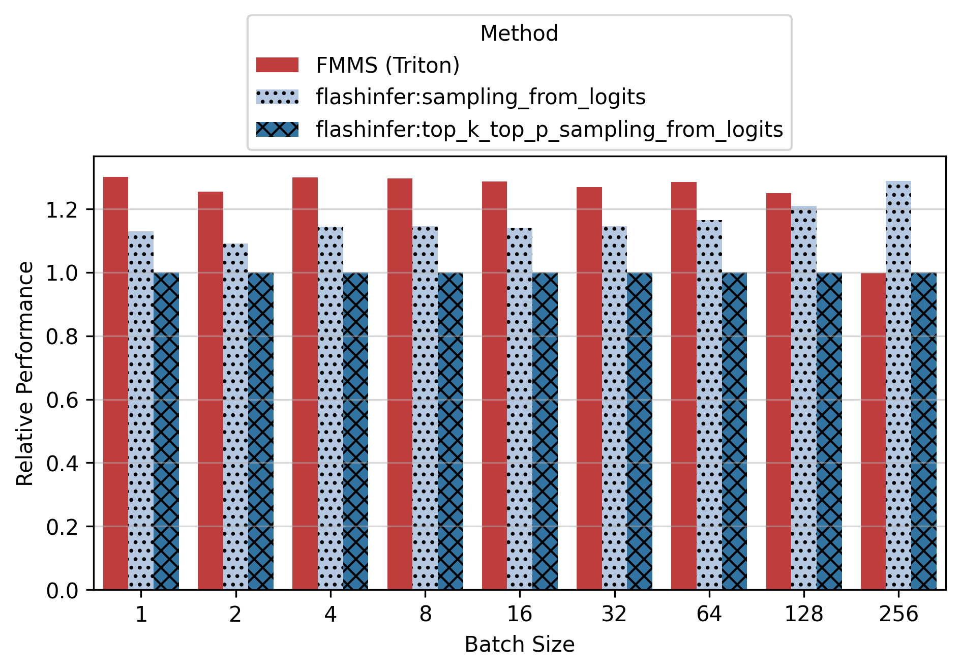
The relative speedup tables show baseline_time / fmms_time, so values > 1.0 mean FMMS is faster.

FlashInfer

Two FlashInfer baselines are compared:

• flashinfer:sampling_from_logits() is FlashInfer’s fastest sampling kernel, but not used in vLLM. It also uses the Gumbel-max trick internally, but operates on pre-materialized logits.
• flashinfer:top_k_top_p_sampling_from_logits() is the sampling function used in vLLM when top-k or top-p is set (I set top-k=-1 and top-p=1.0 to disable filtering).

Small

B300

Figure 3: Relative performance vs FlashInfer baselines on B300.

B200

Relative performance vs FlashInfer baselines on B200.

H200

Relative performance vs FlashInfer baselines on H200.

H100

Relative performance vs FlashInfer baselines on H100.

Show data table: vs top_k_top_p

Speedup vs top_k_top_p (small config). Bold marks the peak speedup per GPU.

GPU / Batch Size	1	2	4	8	16	32	64	128	256
B300	2.05	2.05	1.94	2.24	2.30	2.10	1.89	1.72	1.63
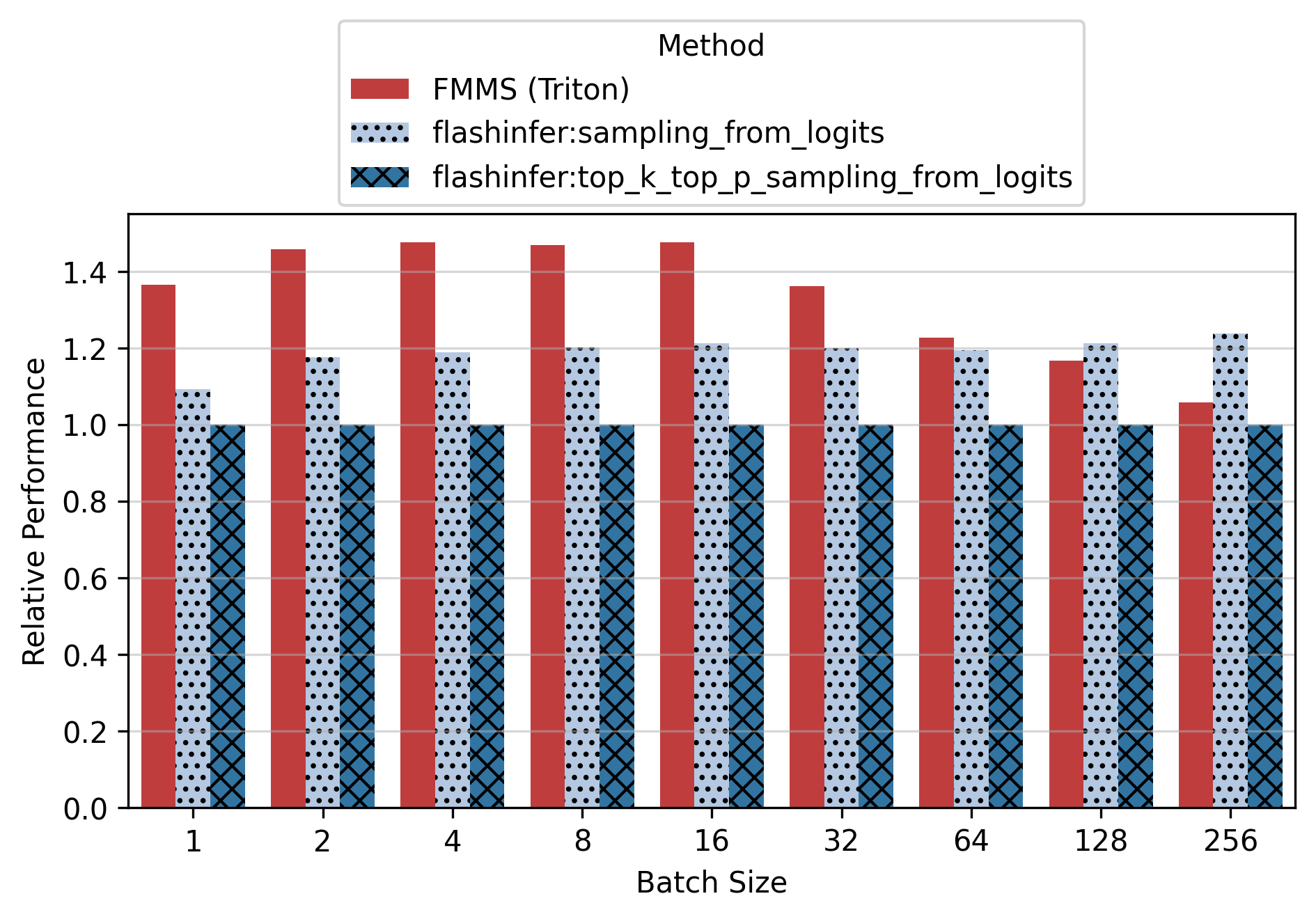
B200	1.36	1.46	1.48	1.47	1.48	1.36	1.23	1.17	1.06
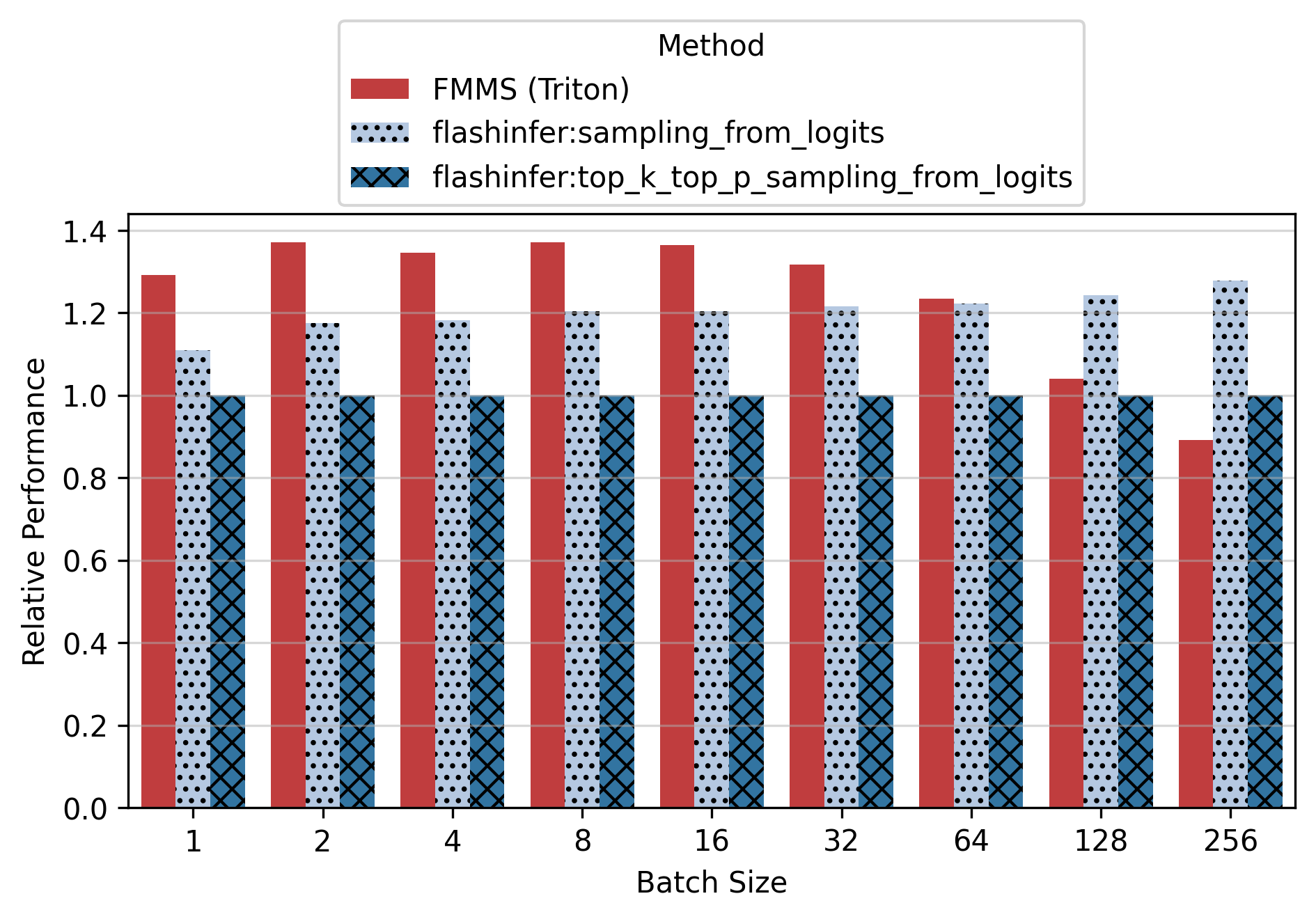
H200	1.29	1.37	1.35	1.37	1.36	1.32	1.23	1.04	0.89
H100	1.30	1.25	1.30	1.30	1.29	1.27	1.29	1.25	1.00

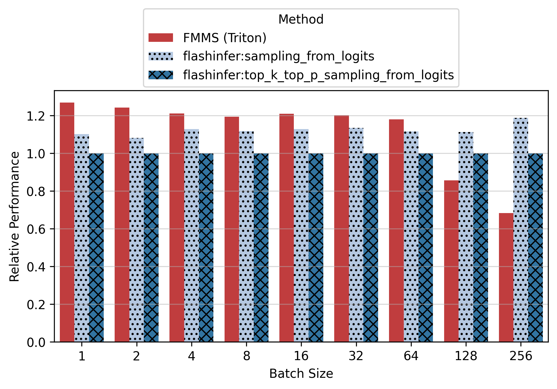
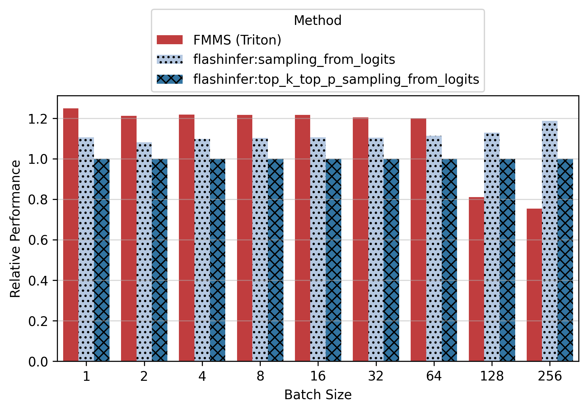
Show data table: vs sampling_from_logits

Speedup vs sampling_from_logits (small config). Bold marks the peak speedup per GPU.

GPU / Batch Size	1	2	4	8	16	32	64	128	256
B300	1.25	1.23	1.24	1.23	1.23	1.14	1.04	1.00	0.89
B200	1.25	1.24	1.24	1.22	1.22	1.14	1.03	0.96	0.85
H200	1.16	1.17	1.14	1.14	1.13	1.08	1.01	0.84	0.70
H100	1.15	1.15	1.13	1.13	1.13	1.11	1.10	1.03	0.77

Large

B300

Relative performance vs FlashInfer baselines on B300.

B200

Relative performance vs FlashInfer baselines on B200.

H200

Relative performance vs FlashInfer baselines on H200.

H100

Relative performance vs FlashInfer baselines on H100.

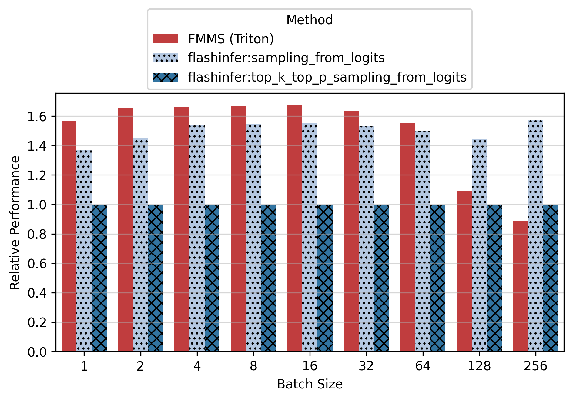
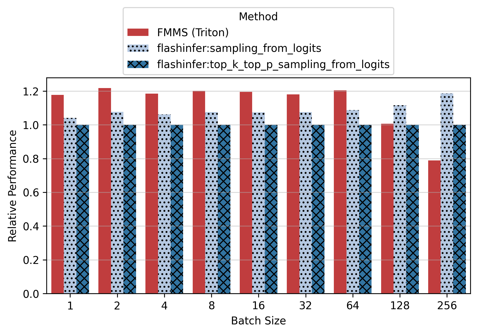
Show data table: vs top_k_top_p

Speedup vs top_k_top_p (large config). Bold marks the peak speedup per GPU.

GPU / Batch Size	1	2	4	8	16	32	64	128	256
B300	1.57	1.65	1.66	1.67	1.67	1.64	1.55	1.09	0.89
B200	1.27	1.24	1.21	1.19	1.21	1.20	1.18	0.86	0.68
H200	1.25	1.21	1.22	1.22	1.22	1.20	1.20	0.81	0.75
H100	1.18	1.22	1.19	1.20	1.20	1.18	1.20	1.01	0.79

Show data table: vs sampling_from_logits

Speedup vs sampling_from_logits (large config). Bold marks the peak speedup per GPU.

GPU / Batch Size	1	2	4	8	16	32	64	128	256
B300	1.14	1.14	1.08	1.08	1.08	1.07	1.03	0.76	0.57
B200	1.15	1.15	1.07	1.07	1.07	1.06	1.06	0.77	0.57
H200	1.13	1.12	1.11	1.10	1.10	1.09	1.08	0.72	0.63
H100	1.13	1.13	1.12	1.12	1.11	1.10	1.11	0.90	0.67

Vs top_k_top_p, FMMS is up to 2.30x faster (B300, small config, N=16). For the small config on B300, FMMS is 1.63-2.30x faster across all batch sizes¹.

Vs sampling_from_logits, FMMS is faster at all batch sizes from 1 to 64 on every GPU tested, with speedups of 3-25%. For the small config, FMMS stays above 1.0x up to N=128 on B300/H100. For the large config, it regresses at N=128+ on most GPUs.

PyTorch Compiled

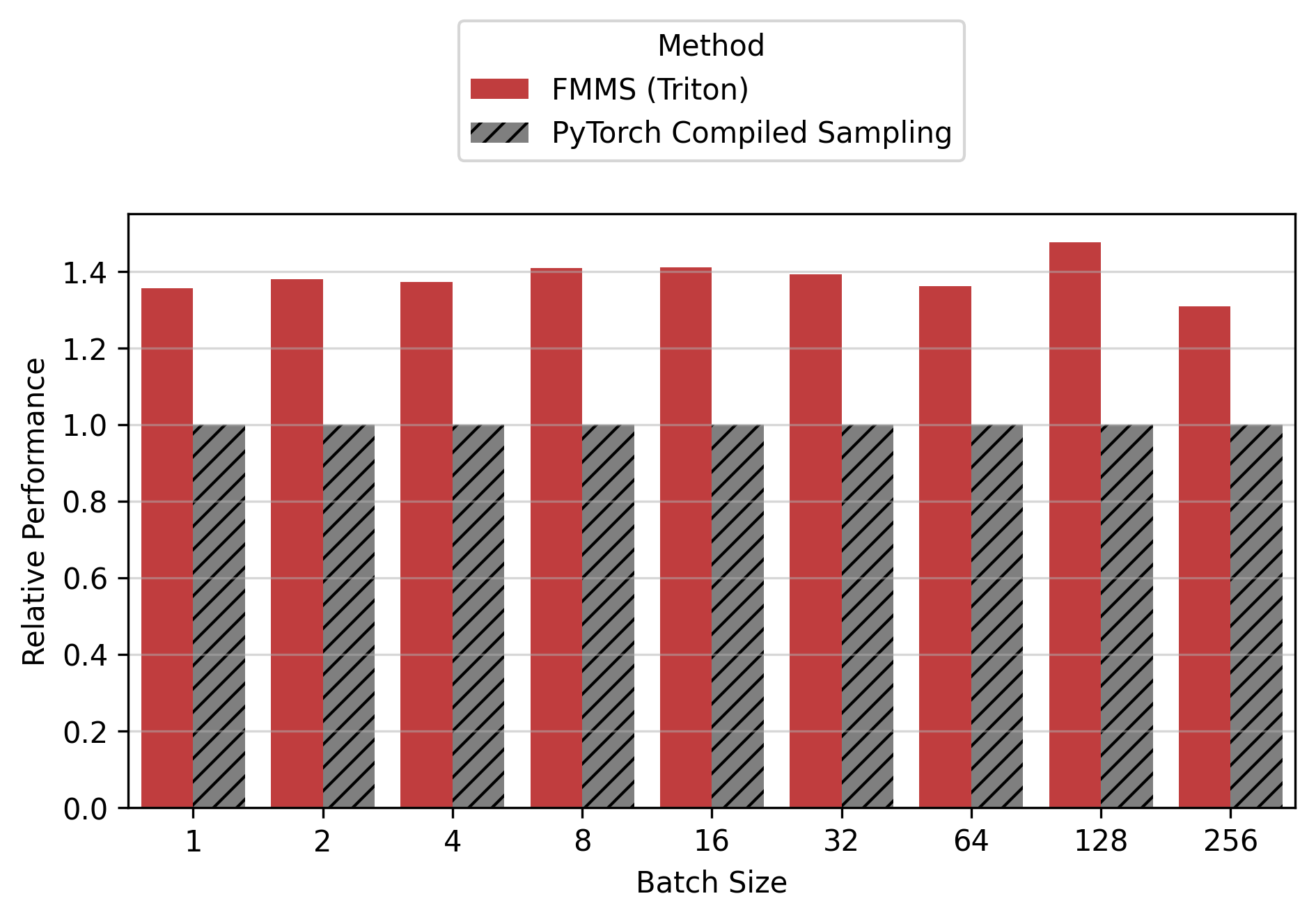
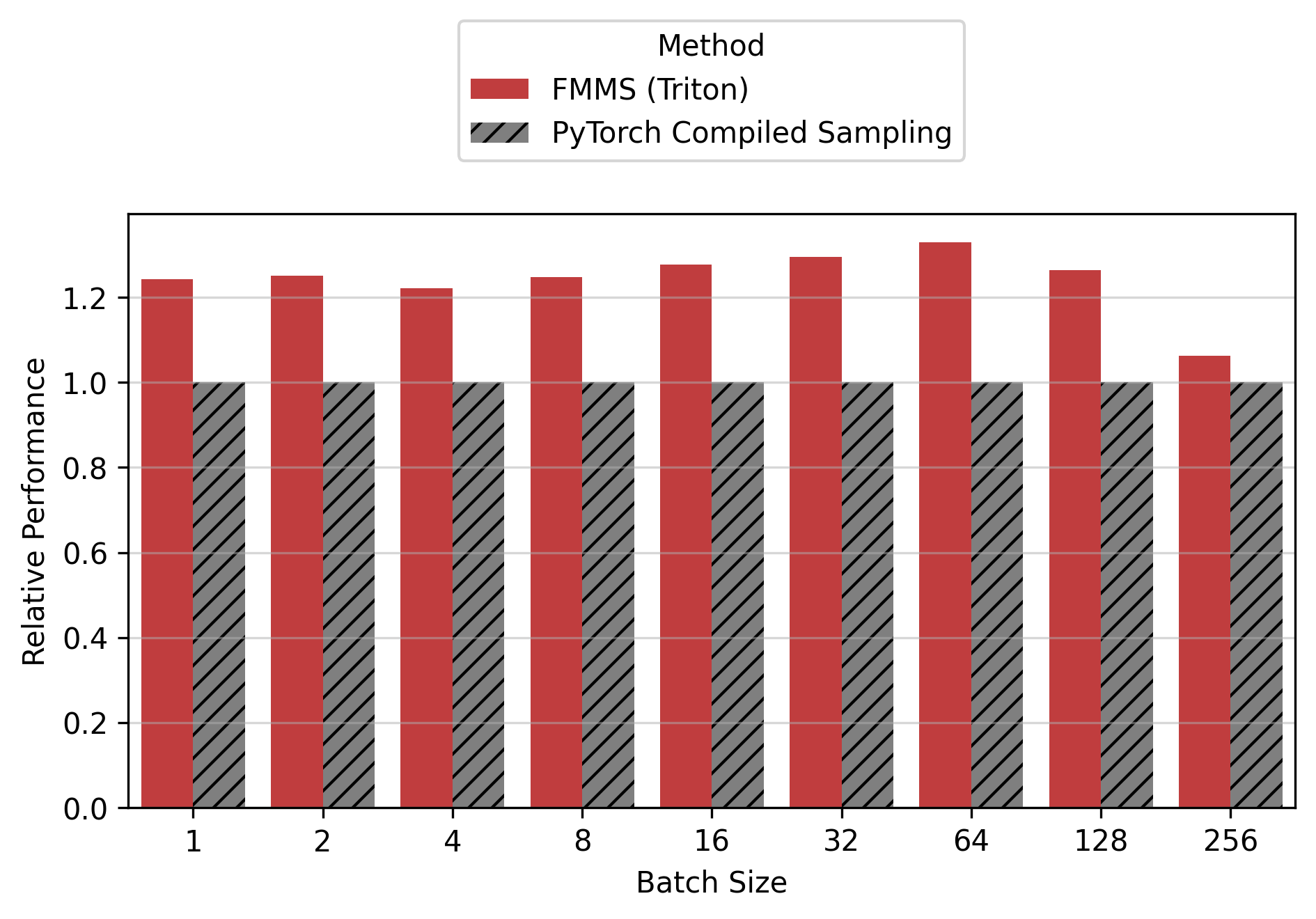
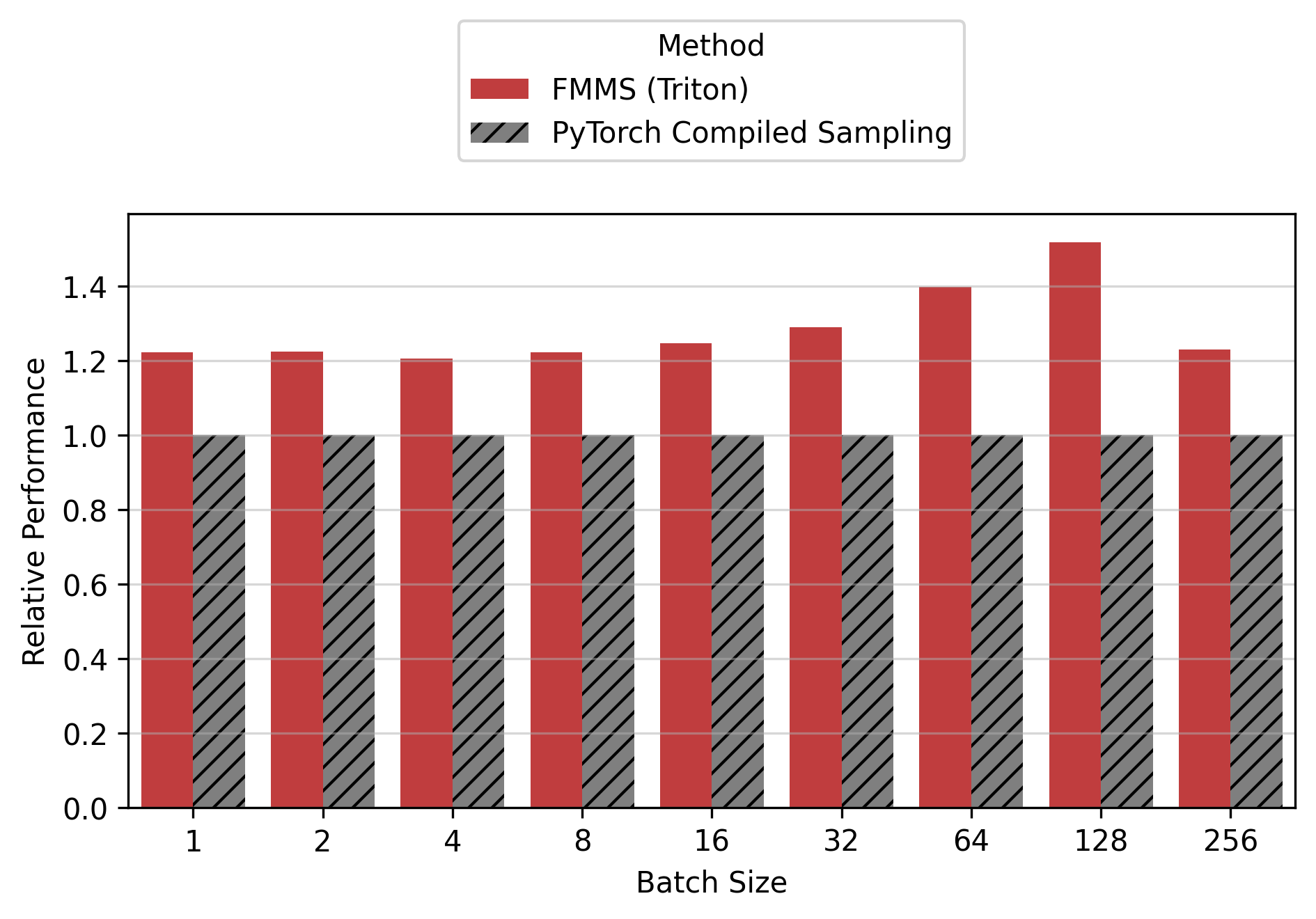
This is the sampling path used in vLLM when top-k and top-p are unset (torch compiled matmul + softmax + torch.multinomial).

Small

B300

Figure 4: Relative performance vs PyTorch Compiled on B300.

B200

Relative performance vs PyTorch Compiled on B200.

H200

Relative performance vs PyTorch Compiled on H200.

H100

Relative performance vs PyTorch Compiled on H100.

Show data table

Speedup vs PyTorch Compiled (small config). Bold marks the peak speedup per GPU.

GPU / Batch Size	1	2	4	8	16	32	64	128	256
B300	1.40	1.38	1.39	1.35	1.43	1.38	1.38	1.48	1.33
B200	1.36	1.38	1.37	1.41	1.41	1.39	1.36	1.48	1.31
H200	1.24	1.25	1.22	1.25	1.28	1.30	1.33	1.26	1.06
H100	1.22	1.23	1.21	1.22	1.25	1.29	1.40	1.52	1.23

Large

B300

Relative performance vs PyTorch Compiled on B300.

B200

Relative performance vs PyTorch Compiled on B200.

H200

Relative performance vs PyTorch Compiled on H200.

H100

Relative performance vs PyTorch Compiled on H100.

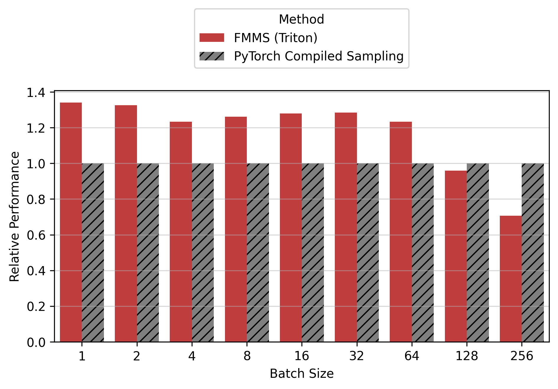
Show data table

Speedup vs PyTorch Compiled (large config). Bold marks the peak speedup per GPU.

GPU / Batch Size	1	2	4	8	16	32	64	128	256
B300	1.34	1.33	1.23	1.26	1.28	1.29	1.23	0.96	0.71
B200	1.35	1.31	1.27	1.24	1.26	1.25	1.27	0.97	0.74
H200	1.26	1.23	1.22	1.22	1.22	1.23	1.28	0.93	0.78
H100	1.22	1.22	1.20	1.21	1.21	1.21	1.28	1.13	0.87

For the small config, FMMS is faster at all batch sizes on all GPUs (minimum 1.06x on H200 at N=256), with speedups of 6-52%. The larger vocab (V=151,936) means more logits traffic, making fusion valuable even at high batch sizes. For the large config, FMMS wins at batch sizes 1-64 (20-35% faster) but regresses at N=128+ on B300/B200/H200. H100 retains its advantage at larger batch sizes than other GPUs: at N=128, it still achieves 1.13x (large) and 1.52x (small). This is likely because H100 has the highest ops:byte ratio (295), keeping the matmul memory-bound longer.

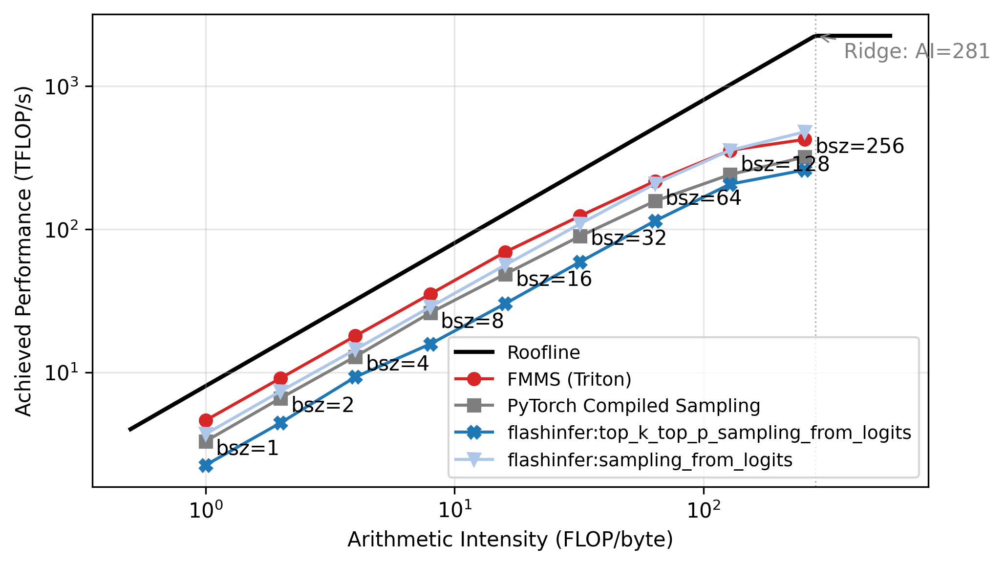
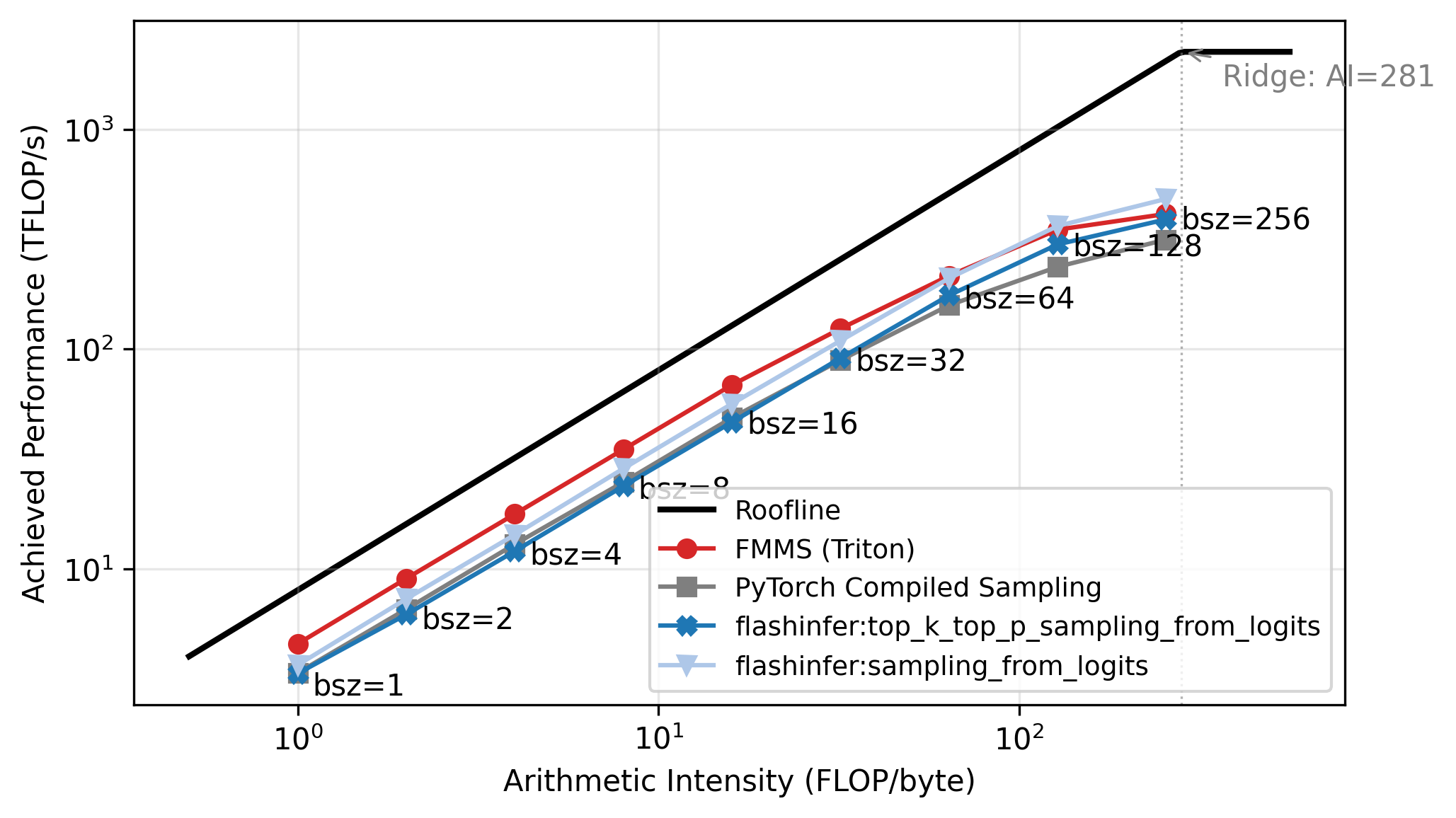
Roofline Analysis

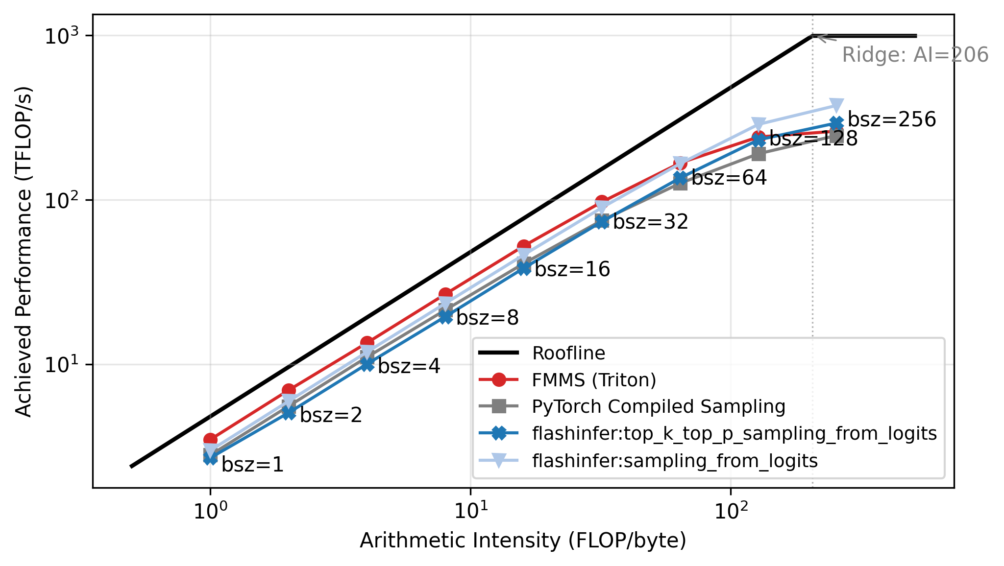
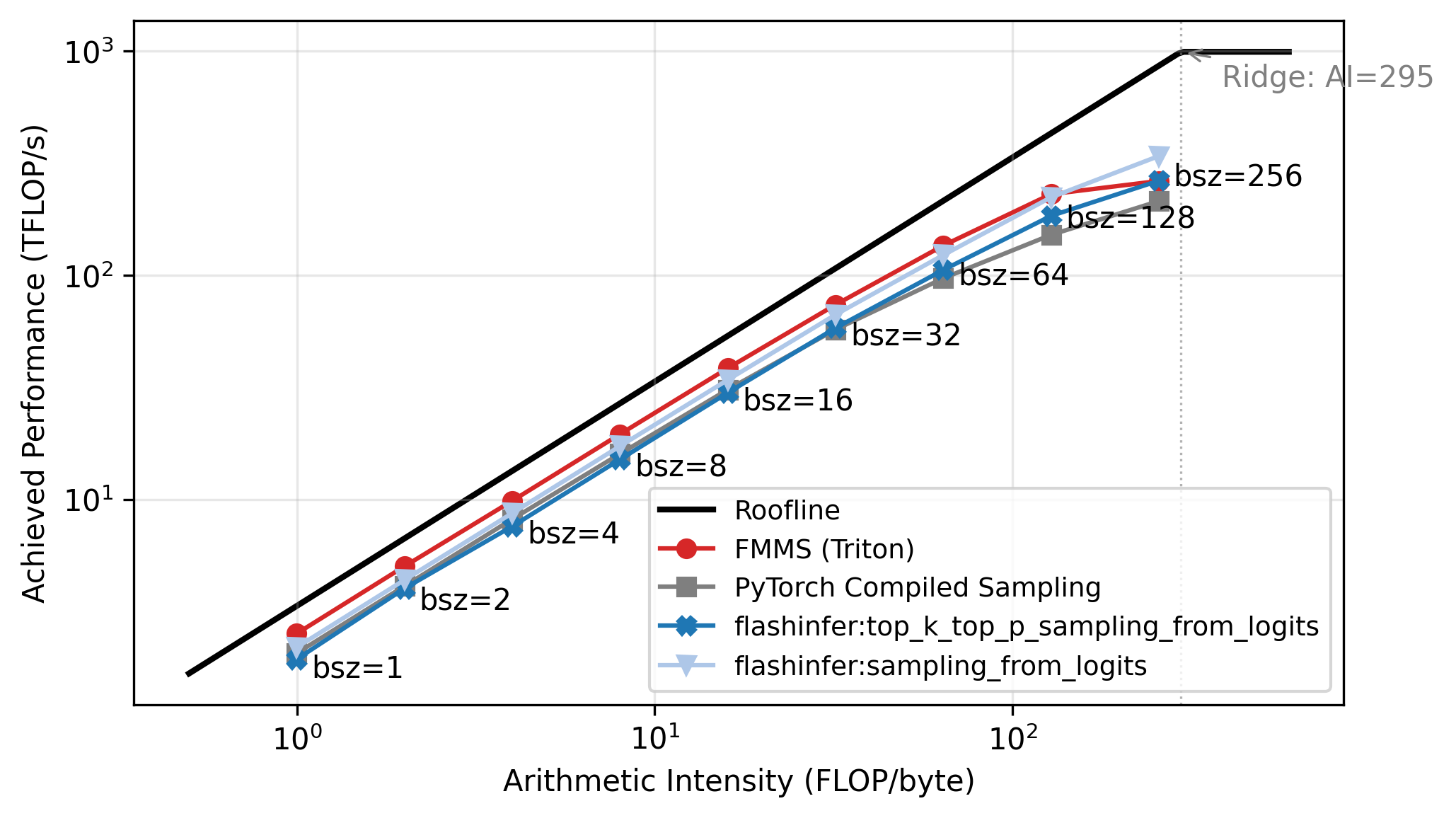
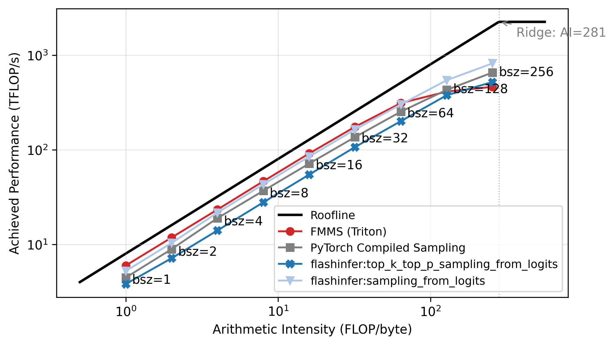
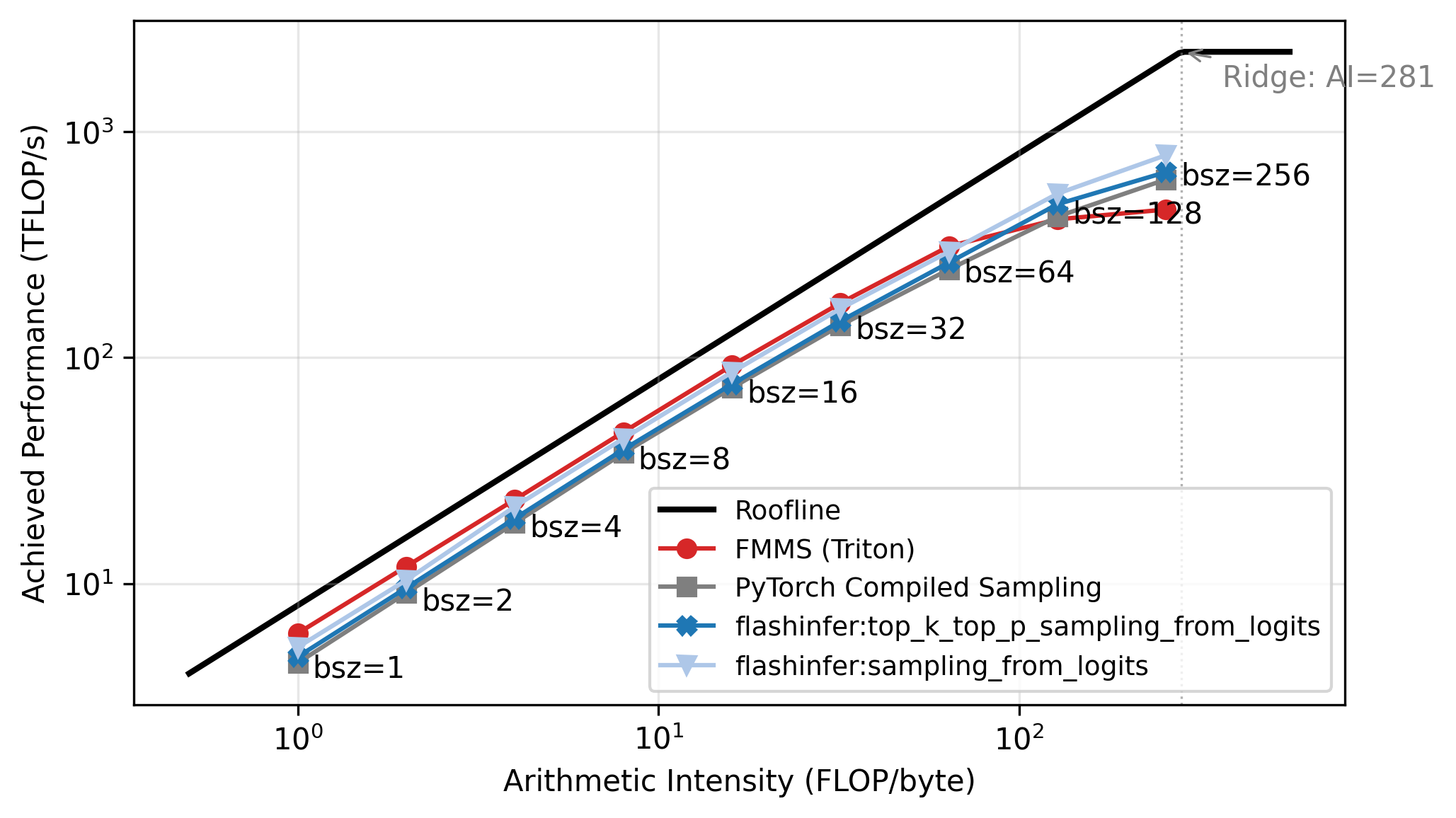
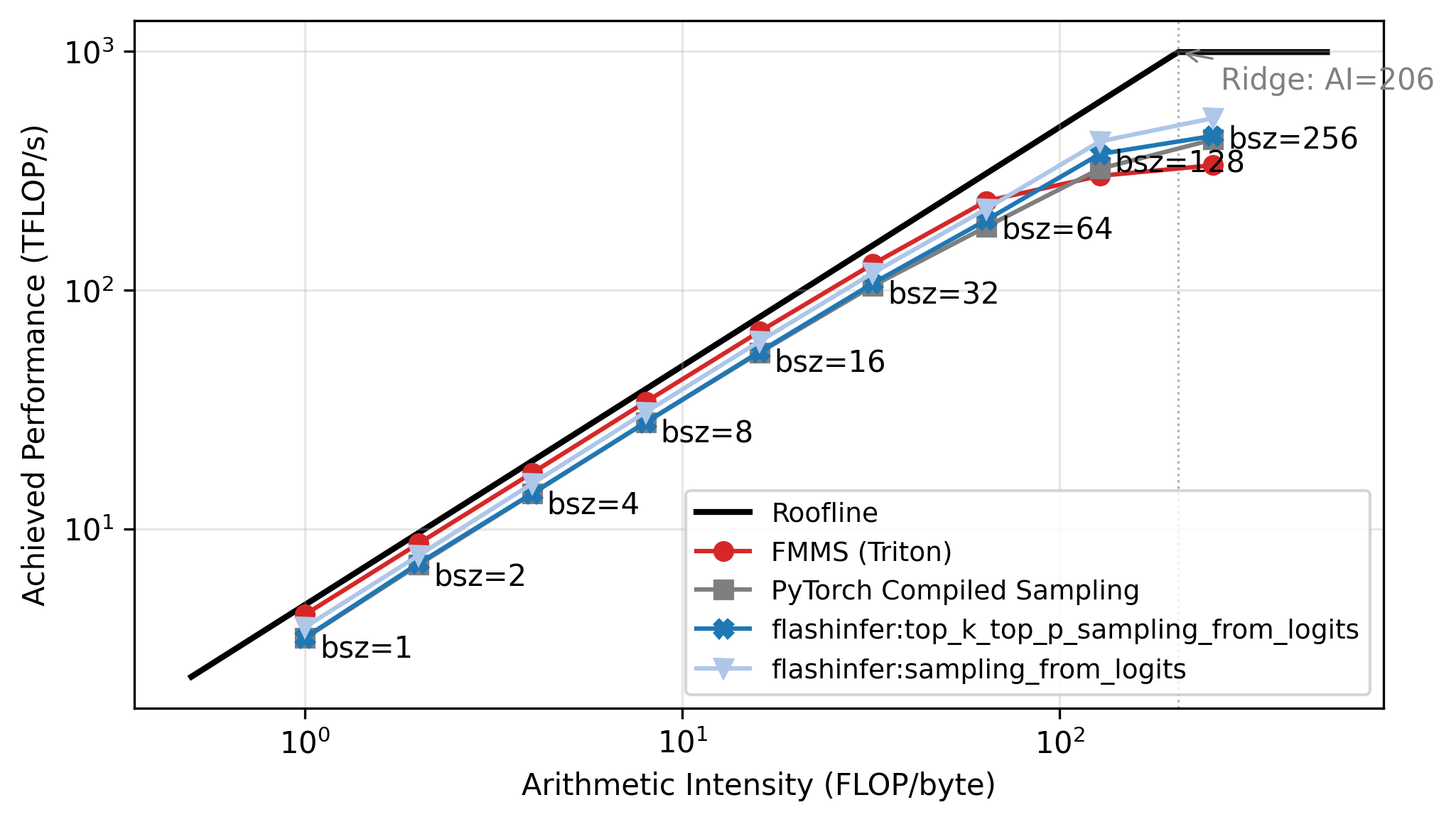
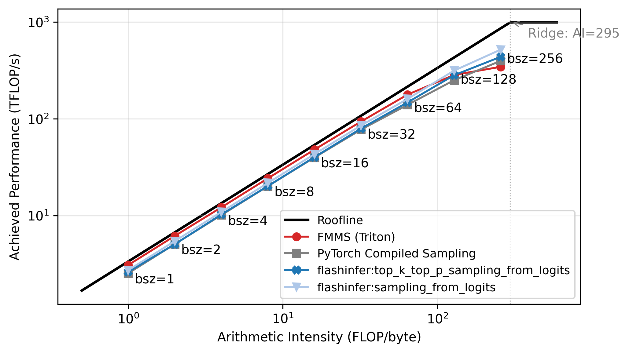
The benchmarks above show a clear crossover: FMMS wins at small batch sizes and regresses at large ones. The explanation lies in the arithmetic intensity of the matmul. The matmul \(W_{[V, d]} \times H_{[N, d]}^T\) has:

\[ \text{Arithmetic Intensity} = \frac{\text{FLOPs}}{\text{Bytes}} = \frac{2 \cdot V \cdot d \cdot N}{2 \cdot V \cdot d} = N \]

The weight matrix \(W\) dominates the memory traffic (\(V \cdot d\) elements, each read once), and the hidden states are negligible when \(N \ll V\)². So the arithmetic intensity is simply \(N\): each byte of weights loaded produces \(N\) multiply-adds.

A GPU becomes compute-bound when the arithmetic intensity exceeds its ops:byte ratio (peak compute / peak memory bandwidth). For the H100:

\[ \text{ops:byte} = \frac{989 \text{ TFLOP/s (BF16)}}{3.35 \text{ TB/s (HBM3)}} \approx 295 \]

The roofline plot in Figure 5 confirms this: all methods track the memory-bound slope up to N=64, then flatten as they approach the compute ceiling. Each point is labeled with its batch size. FMMS sits slightly above the baselines in the memory-bound region because it reads the weight matrix once and writes only two scalars per tile to GMEM, while the baselines write and read back the full logits tensor. At large batch sizes the matmul becomes compute-bound, and the baselines benefit from cuBLAS (via torch.compile), while FMMS implements the matmul in Triton. FMMS also has higher register pressure from fusing Gumbel noise generation into the same kernel.

Small

B300

Figure 5: Roofline model on B300 (V=151,936, d=4,096). The ridge point marks the transition from memory-bound to compute-bound.

B200

Roofline model on B200.

H200

Roofline model on H200.

H100

Roofline model on H100.

Large

B300

Roofline model on B300 (V=128,256, d=8,192).

B200

Roofline model on B200.

H200

Roofline model on H200.

H100

Roofline model on H100.

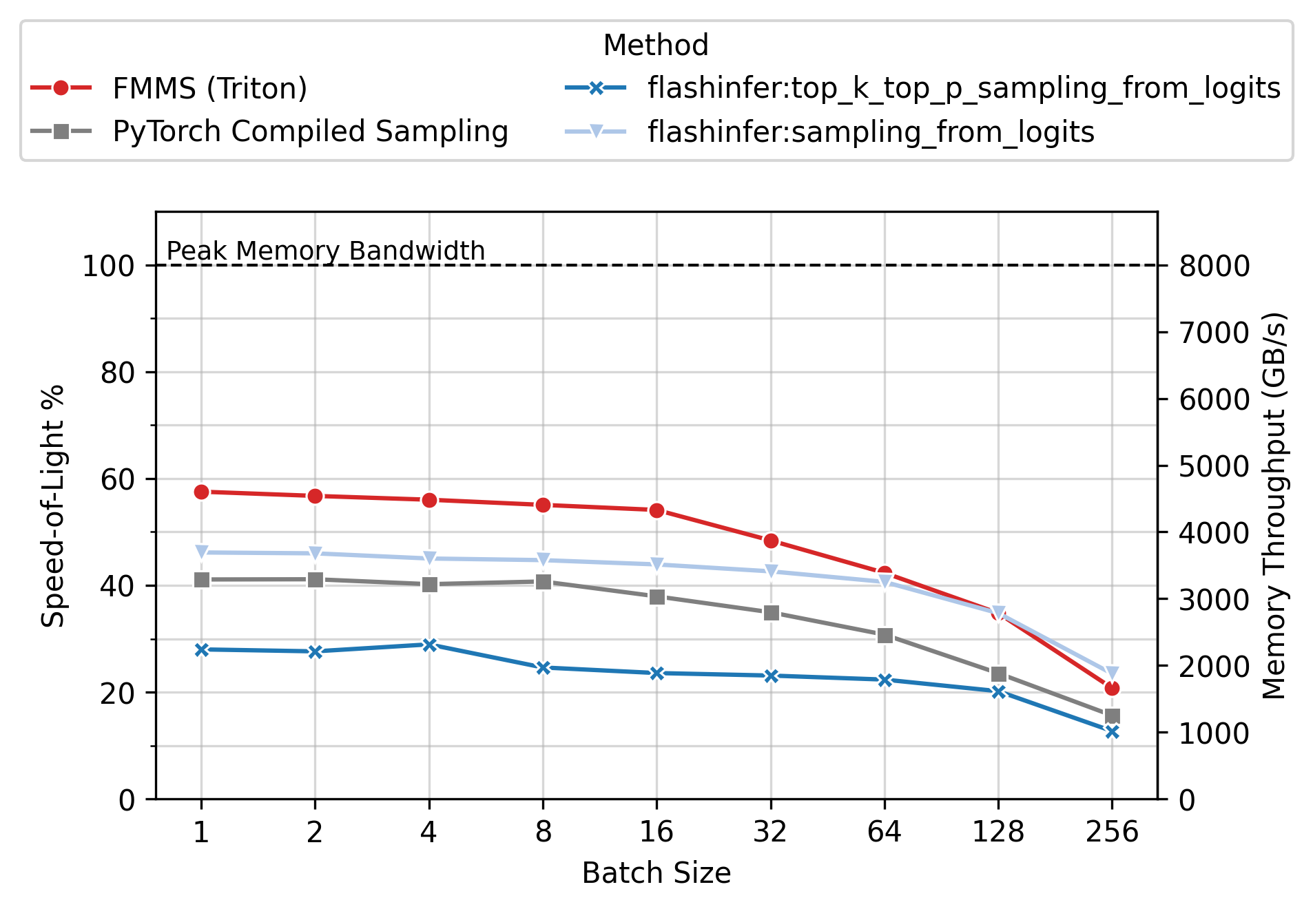
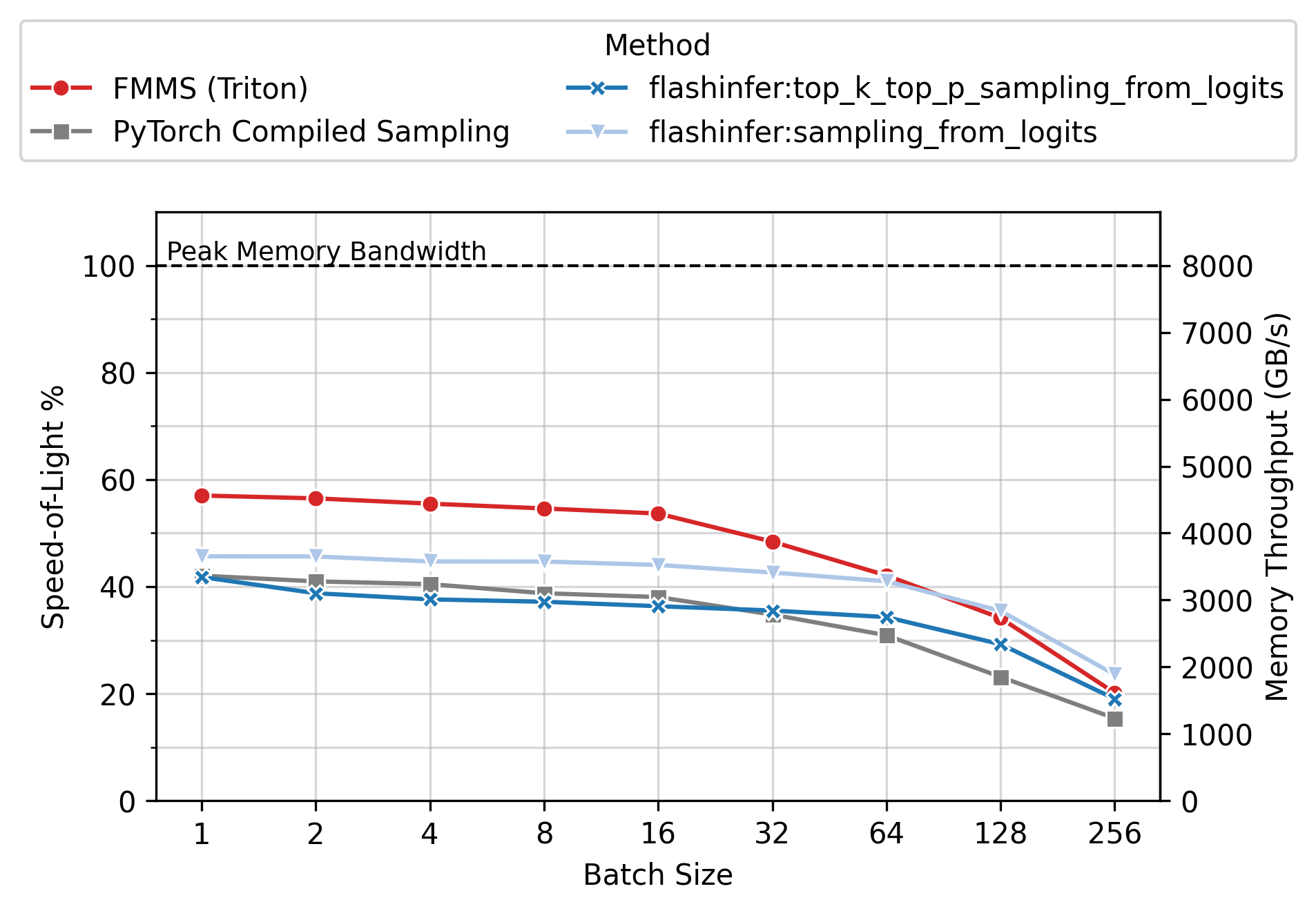
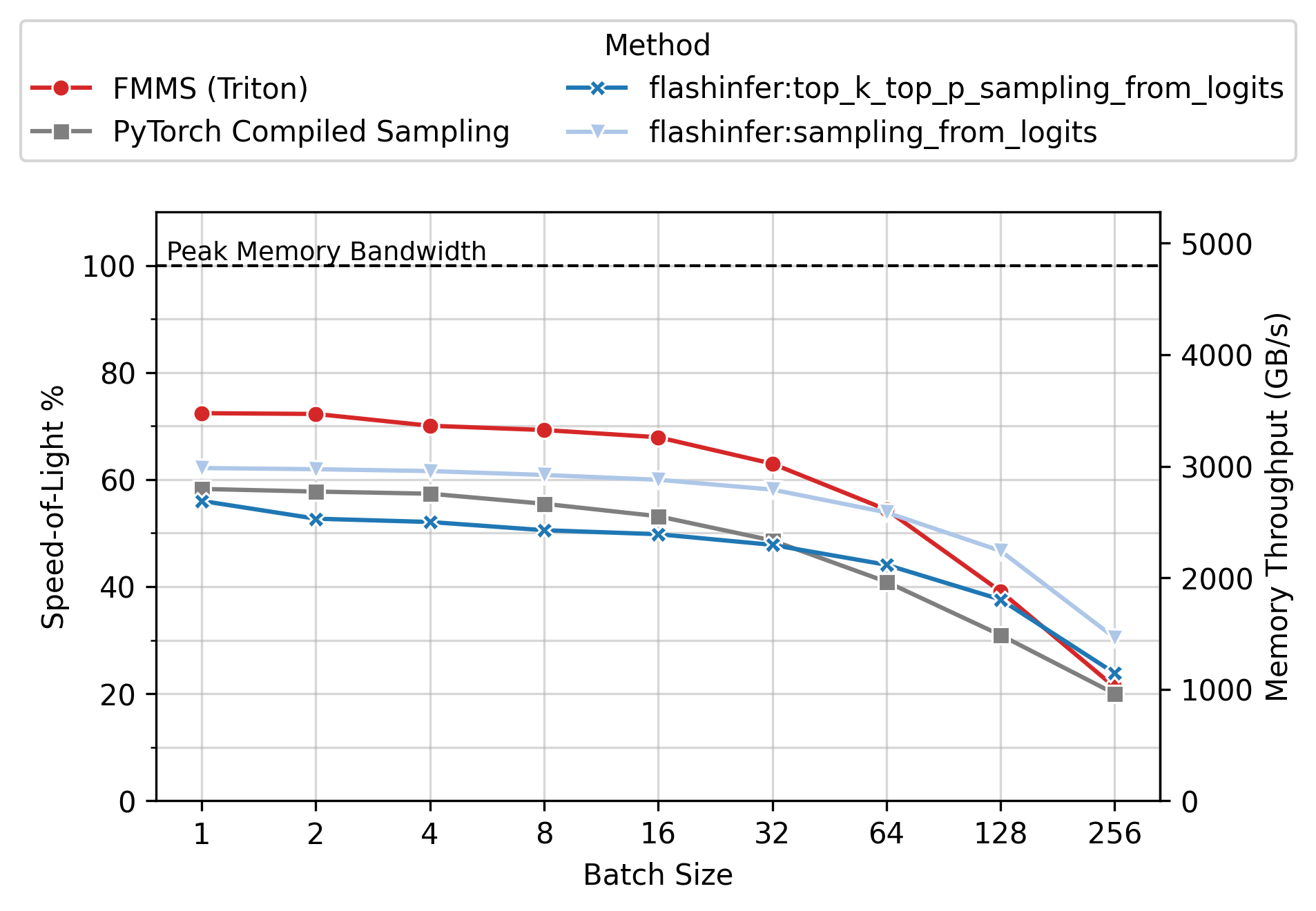
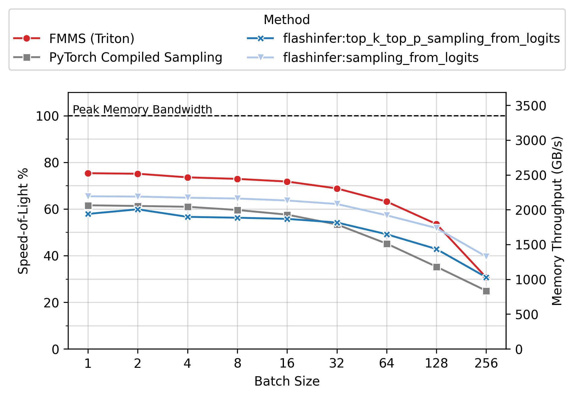
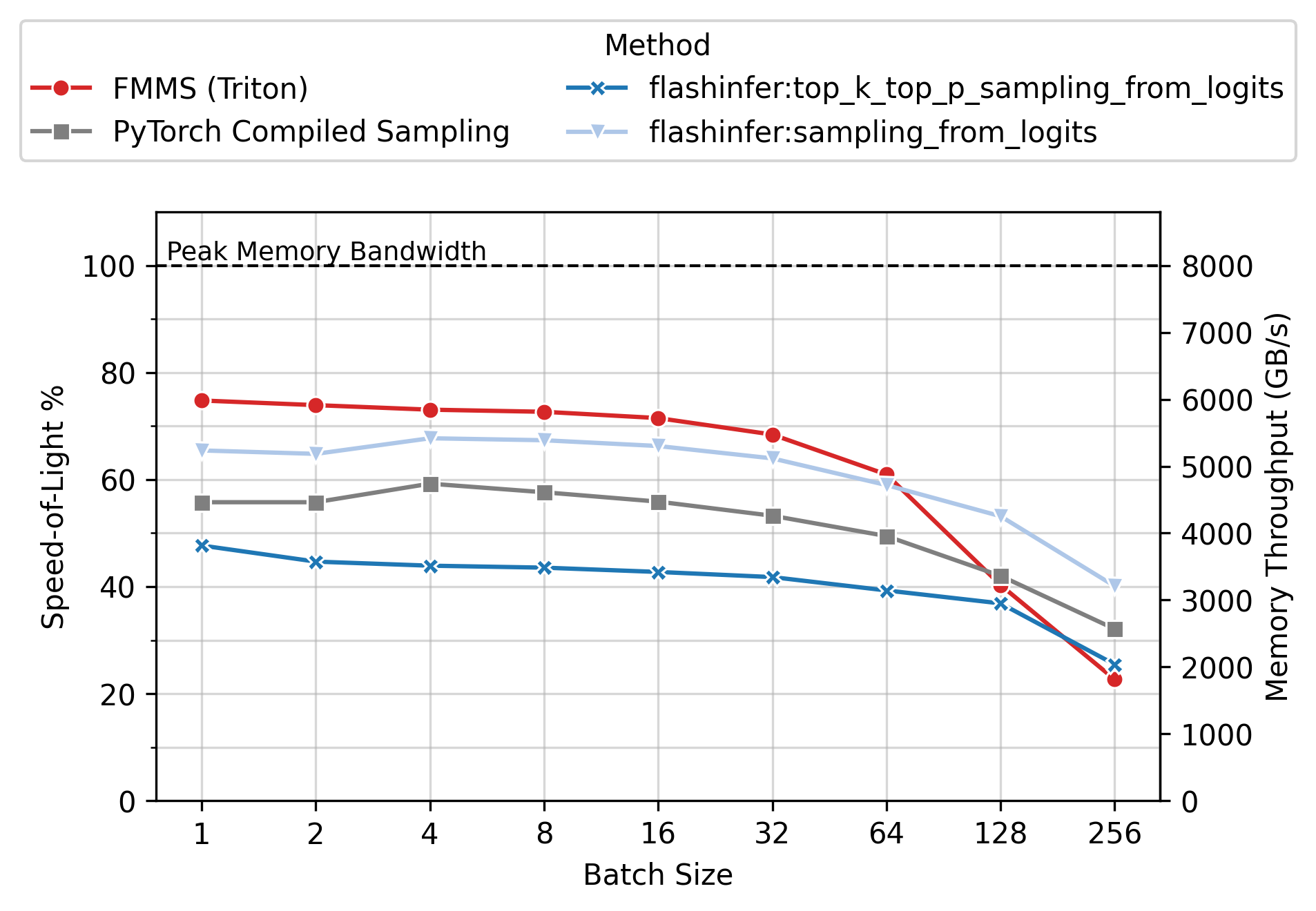
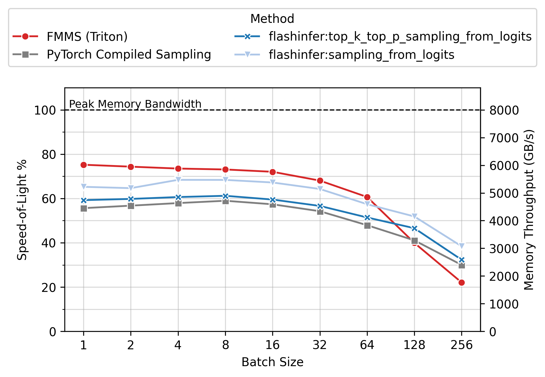
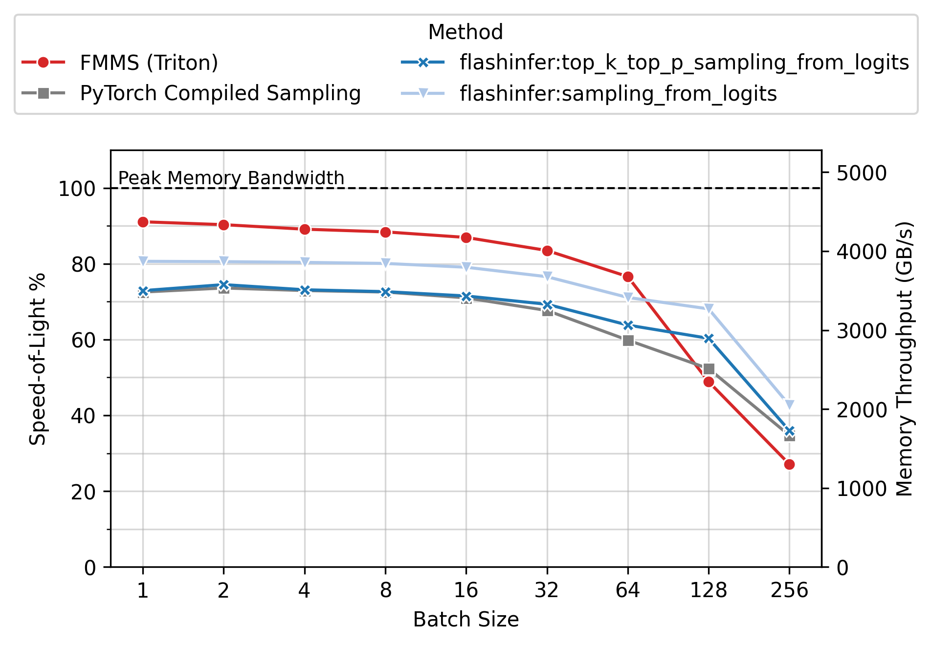
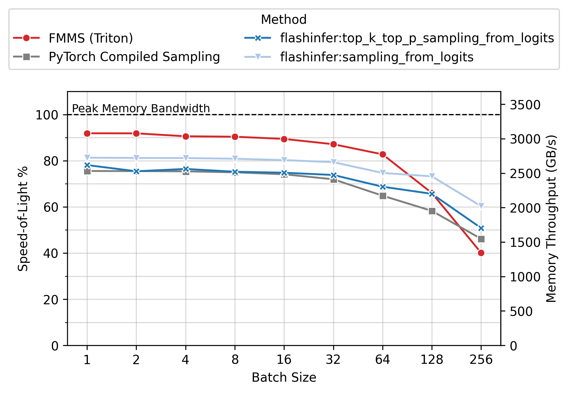
Memory Throughput

Figure 6 shows the achieved memory throughput (GB/s) as a function of batch size. At low batch sizes (N \(\leq\) 64), where the operation is deeply memory-bound, FMMS consistently achieves higher throughput than all baselines. Peak SoL varies by GPU and config: up to ~90% on H100/H200 (large config), ~55-60% on B300/B200 (small config). 100% would mean the kernel does nothing but stream the weight matrix from GMEM at the hardware’s maximum rate, with zero overhead for computation, synchronization, or memory access patterns.

Small

B300

Figure 6: Memory throughput on B300 (V=151,936, d=4,096). The dashed line shows peak HBM bandwidth.

B200

Memory throughput on B200.

H200

Memory throughput on H200.

H100

Memory throughput on H100.

Large

B300

Memory throughput on B300 (V=128,256, d=8,192).

B200

Memory throughput on B200.

H200

Memory throughput on H200.

H100

Memory throughput on H100.

End-to-End Benchmarks (vLLM)

The kernel benchmarks measure the FMMS kernel in isolation. To measure end-to-end impact, I integrated FMMS into vLLM (branch) and benchmarked median time per output token (TPOT) across concurrency levels using vllm bench sweep. I chose four models spanning different sizes and architectures. The LM head is a standard dense linear layer in all four, so FMMS applies identically regardless of MoE routing.

Model	Type	Hidden size (d)	Vocab size (V)
gpt-oss-120b	MoE (128 experts, 4 active)	2,880	201,088
Qwen3-1.7B	Dense	2,048	151,936
Qwen3-8B	Dense	4,096	152,064
Qwen3-32B	Dense	5,120	152,064

The “Baseline” in the tables below is vLLM’s default sampling path (torch compiled matmul followed by softmax and torch.multinomial), without FMMS. Each configuration is run 5 times per trial; some models have 2 independent trials to increase confidence. The plots pool data from all trials, and per-trial tables are available in the collapsible sections. All results are on a B200 GPU with PyTorch 2.10.0 and CUDA 13.0, run on Modal.

gpt-oss-120b

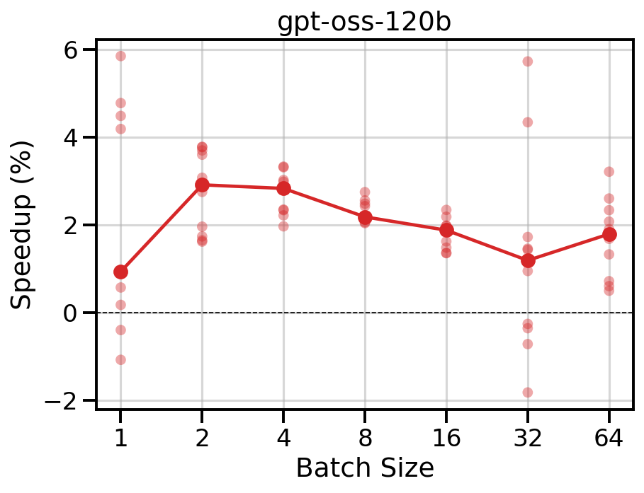
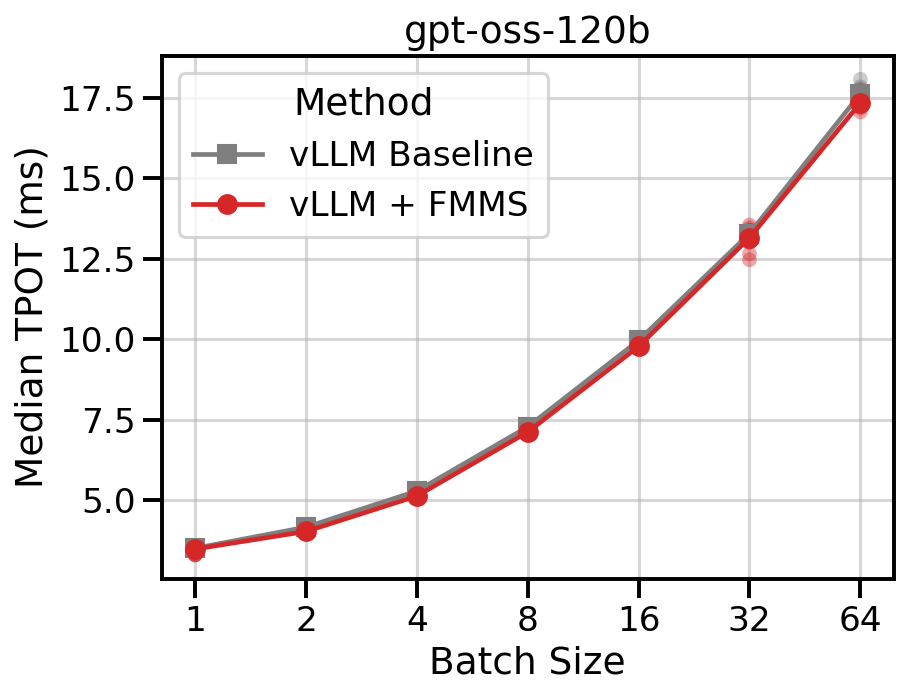
The LM head is a smaller fraction of the total decode step in a 120B-parameter model. FMMS reduces TPOT by up to 5% at low concurrency (1-8), with modest 1-2% improvements at higher concurrency levels.

Data table

Trial 1

Median TPOT on gpt-oss-120b, trial 1. Bold marks the peak reduction.

Concurrency	Baseline (ms)	FMMS Triton (ms)	TPOT Reduction
1	3.45	3.29	-4.6%
2	4.14	3.99	-3.6%
4	5.28	5.11	-3.2%
8	7.30	7.12	-2.5%
16	9.94	9.77	-1.7%
32	13.34	13.39	+0.4%
64	17.80	17.50	-1.7%

Trial 2

Median TPOT on gpt-oss-120b, trial 2. Bold marks the peak reduction.

Concurrency	Baseline (ms)	FMMS Triton (ms)	TPOT Reduction
1	3.54	3.53	-0.3%
2	4.17	4.11	-1.4%
4	5.28	5.15	-2.5%
8	7.27	7.12	-2.1%
16	9.97	9.79	-1.8%
32	13.23	13.03	-1.5%
64	17.52	17.24	-1.6%

Qwen3-1.7B

The small hidden dimension makes the LM head matmul strongly memory-bound, so fusion has a large impact. FMMS reduces TPOT by 11-19% across all concurrency levels.

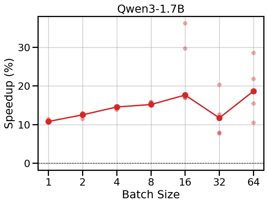
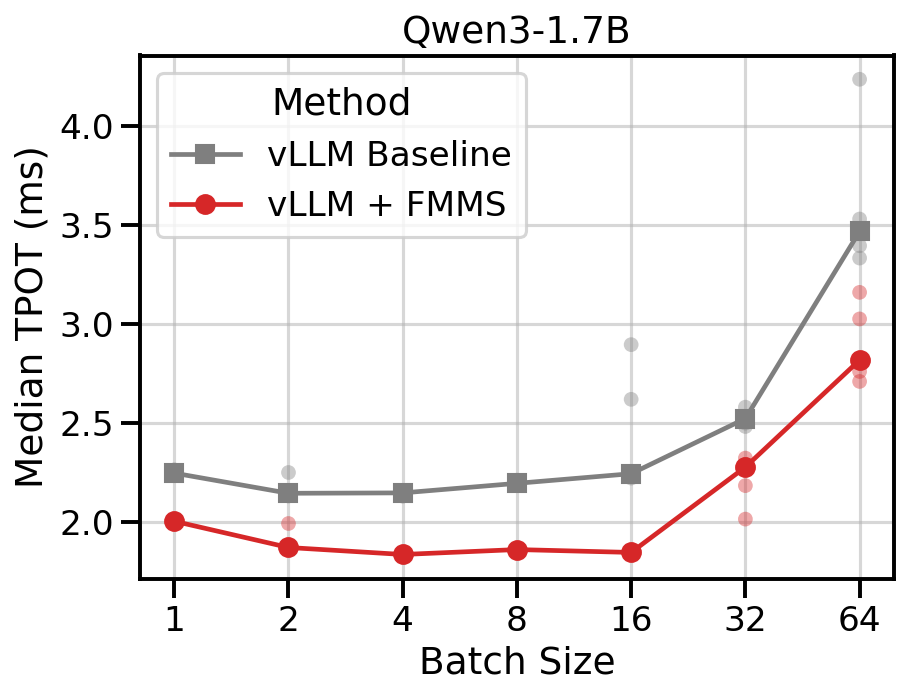
Data table

Median TPOT on Qwen3-1.7B. Bold marks the peak reduction.

Concurrency	Baseline (ms)	FMMS Triton (ms)	TPOT Reduction
1	2.25	2.00	-10.8%
2	2.14	1.87	-12.5%
4	2.15	1.84	-14.6%
8	2.19	1.86	-15.2%
16	2.24	1.85	-17.7%
32	2.52	2.28	-11.7%
64	3.47	2.82	-18.7%

Qwen3-8B

FMMS reduces TPOT by 3-7% at most concurrency levels, with larger gains in some runs (up to 17% at concurrency 32 in trial 1).

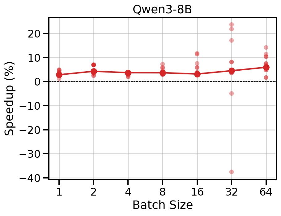
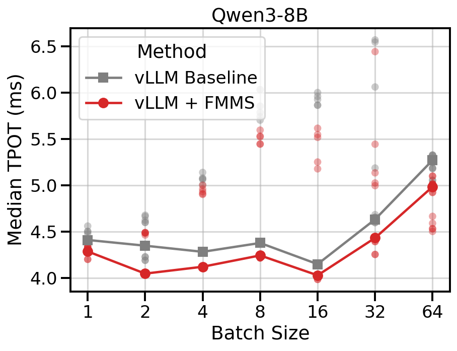
Data table

Trial 1

Median TPOT on Qwen3-8B, trial 1. Bold marks the peak reduction.

Concurrency	Baseline (ms)	FMMS Triton (ms)	TPOT Reduction
1	4.50	4.34	-3.8%
2	4.63	4.49	-3.5%
4	5.07	4.93	-2.7%
8	5.79	5.53	-5.6%
16	5.93	5.52	-7.5%
32	6.06	5.14	-17.1%
64	5.06	4.53	-10.4%

Trial 2

Median TPOT on Qwen3-8B, trial 2. Bold marks the peak reduction.

Concurrency	Baseline (ms)	FMMS Triton (ms)	TPOT Reduction
1	4.41	4.29	-2.8%
2	4.35	4.05	-6.9%
4	4.28	4.12	-3.7%
8	4.38	4.22	-3.6%
16	4.15	4.02	-2.9%
32	4.63	4.43	-4.5%
64	5.29	5.01	-5.7%

Qwen3-32B

FMMS reduces TPOT by 1-2% across concurrency levels.

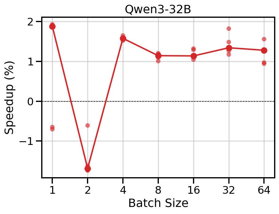
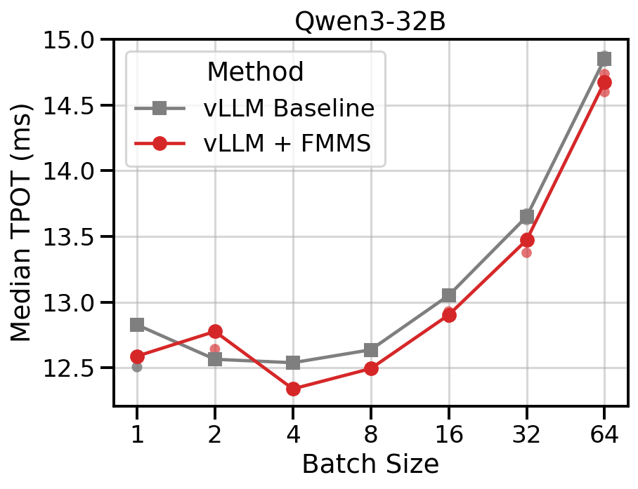
Data table

Median TPOT on Qwen3-32B.

Concurrency	Baseline (ms)	FMMS Triton (ms)	TPOT Reduction
1	12.83	12.59	-1.9%
2	12.56	12.78	+1.7%
4	12.54	12.34	-1.6%
8	12.64	12.49	-1.1%
16	13.05	12.90	-1.1%
32	13.65	13.47	-1.3%
64	14.85	14.68	-1.3%

A Note on Variability

The Qwen3-8B trials show substantial run-to-run variability: at concurrency 32, trial 1 measures a 17% reduction, while trial 2 measures a 4.5% reduction. The absolute runtimes differ by 30%, potentially due to GPU thermal state or other system-level factors. This variability is inherent to end-to-end serving benchmarks, where many system-level factors beyond the kernel itself affect TPOT. Despite this, the direction is consistent: FMMS outperforms the baseline at every concurrency level in both trials.

Correctness

FMMS uses the Gumbel-max trick, which produces exact samples from the categorical distribution, not an approximation. But because the output is stochastic, correctness is harder to verify than for a deterministic kernel. You cannot compare the output to a reference value; instead, you need statistical tests that verify the output distribution is correct.

I verify this with a chi-squared goodness-of-fit test that runs as a regular unit test during development: draw 10,000 samples from the kernel using synthetic inputs with known logit vectors, and compare the empirical token frequencies against the theoretical softmax probabilities. The test is parametrized over multiple vocabulary sizes and batch sizes to catch tile-boundary edge cases.

End-to-End: GSM8K

As an end-to-end quality check, I integrated FMMS into vLLM and ran the GSM8K benchmark (1,319 questions, 0-shot chain-of-thought) via lm-evaluation-harness on Qwen3-1.7B. Answers were graded by an LLM judge.

GSM8K accuracy on Qwen3-1.7B

Variant	Accuracy	95% CI
Baseline (vLLM default)	89.6%	[87.9%, 91.2%]
FMMS Triton	89.4%	[87.7%, 91.0%]

To test whether this 0.2 percentage point difference is meaningful, I use a paired bootstrap test (10,000 resamples). The test is paired because both variants answer the same 1,319 questions: it computes per-question differences (correct vs. incorrect), then bootstraps the mean difference. This cancels out shared question difficulty and focuses on questions where the variants actually disagree. The result is p=0.776, far from significant (threshold: p < 0.05), confirming that FMMS does not degrade model accuracy.

The Algorithm

The matmul \(W_{[V,d]} \times H_{[N,d]}^T\) is tiled across the \(V\), \(d\), and \(N\) dimensions as shown in Figure 7. Each tile produces a \((T_V, T_N)\) block of logits in SRAM.

Figure 7: Tiling the computation of the logits.

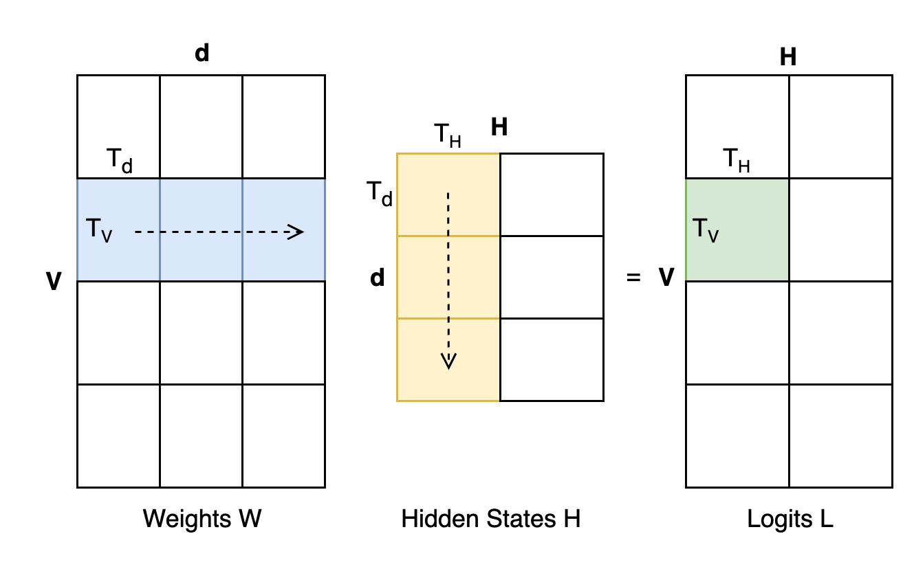
Since argmax decomposes over tiles (as described above), the kernel has a two-stage design:

• Stage 1 (Triton kernel): A 2D grid of programs indexed by (v, h) (vocabulary tile, batch tile). Each program computes its logit tile, scales by temperature, adds Gumbel noise, and finds the tile-local maximum. Only the max value and its global vocabulary index are written to GMEM.
• Stage 2 (host-side reduction): A cheap PyTorch reduction over the num_V_tiles local maxima per hidden state:

best_tiles = tile_maxs.argmax(dim=0)   # which tile won?
samples = tile_indices.gather(0, best_tiles)  # what index did it have?

Stage 1: Per-Tile Logic

Here is what each program in the 2D grid does, in pseudocode:

def program(v_tile, h_tile, W, H, temperature, seed):
    logits = zeros(T_V, T_N, dtype=float32)
1    for d_start in range(0, d, T_d):
        w = W[v_tile, d_start : d_start + T_d]      # load [T_V, T_d] from GMEM
        h = H[h_tile, d_start : d_start + T_d]      # load [T_N, T_d] from GMEM
        logits += w @ h.T                           # accumulate in SRAM

    logits = logits / temperature
2    U = rand(T_V, T_N)
    gumbel_noise = -log(-log(U))
    noised = logits + gumbel_noise

3    max_val, max_idx = max(noised, dim=V)
    GMEM_maxs[v_tile, h_tile] = max_val             # [T_N]
    GMEM_idxs[v_tile, h_tile] = max_idx

1

The inner loop tiles the \(d\) dimension. Each iteration loads one strip of \(W\) and \(H\) and accumulates a partial dot product. The full logit tile never leaves SRAM.

2

Gumbel noise is generated in-kernel using Triton’s Philox PRNG (tl.rand), one draw per logit element. Each (v, h) tile uses a different seed offset so tiles produce independent noise.

3

The argmax over the \(V\) dimension reduces the \((T_V, T_N)\) tile to just \(T_N\) values. The full logit tile is consumed and discarded in SRAM.

Related Work

Cut Your Losses in Large-Vocabulary Language Models (Wijmans et al. 2025) is the direct inspiration for this work. They avoid materializing logits during training by computing the cross-entropy loss incrementally on SRAM, reducing memory from 24GB to 1MB for Gemma 2 (2B). FMMS extends this idea to inference, where the challenge shifts from loss computation to sampling.

FlashSampling (Qin et al. 2025) presents a conceptually very similar algorithm for fused sampling. The paper was submitted to ICLR 25 but was not accepted, and no open-source implementation is available.

FlashInfer (Ye et al. 2025) provides high-performance sampling kernels used in vLLM (Kwon et al. 2023) and SGLang (Zheng et al. 2024), but all its sampling functions take pre-materialized logits or probabilities as input. Liger Kernel (Hsu et al. 2025) focuses on training-time kernel fusion and includes no sampling primitives. The online-softmax method (Milakov and Gimelshein 2018) enables incremental normalization and is used in FlashAttention (Dao et al. 2022), but neither applies it to sampling from the LM head.

Conclusion

FMMS is most effective when the LM head matmul is memory-bound: batch sizes 1-64, which covers the typical LLM decode regime. In this range, it outperforms every baseline on every GPU tested, with kernel-level speedups of up to 25% vs FlashInfer’s fastest sampling kernel and 20-52% vs PyTorch compiled sampling. At larger batch sizes (128+), the matmul becomes compute-bound and cuBLAS-backed baselines are faster.

The end-to-end impact depends on how much of the decode step the LM head represents. For small models (Qwen3-1.7B), FMMS reduces TPOT by up to 19%. For large models (gpt-oss-120b, Qwen3-32B), the LM head is a smaller fraction of the total step, so improvements are modest (1-5%). The sweet spot is small-to-medium models served at low-to-moderate concurrency, where the LM head is a significant bottleneck and the matmul stays memory-bound.

The code is open-source at github.com/tomasruizt/fused-mm-sample. FMMS is currently integrated into vLLM on a feature branch, not merged upstream.

Future Work

Top-k/top-p filtering. FMMS does not yet support top-k or top-p filtering, but it is possible to implement them. For Top-k: each tile can compute a local top-k during the matmul, and a small merge step combines the per-tile candidates. Top-p can be implemented if it is applied after top-k, as is done in the FlashInfer top-k-top-p kernel, and also on the vLLM PyTorch sampling path. In this case, top-p filtering is applied only to the surviving top-k tokens.

References

Dao, Tri, Daniel Y Fu, Stefano Ermon, Atri Rudra, and Christopher Re. 2022. “FlashAttention: Fast and Memory-Efficient Exact Attention with IO-Awareness.” In Advances in Neural Information Processing Systems, edited by Alice H. Oh, Alekh Agarwal, Danielle Belgrave, and Kyunghyun Cho. https://openreview.net/forum?id=H4DqfPSibmx.

Hsu, Pin-Lun, Yun Dai, Vignesh Kothapalli, Qingquan Song, Shao Tang, Siyu Zhu, Steven Shimizu, Shivam Sahni, Haowen Ning, and Yanning Chen. 2025. “Liger Kernel: Efficient Triton Kernels for LLM Training.” https://arxiv.org/abs/2410.10989.

Huijben, I. A. M., W. Kool, M. B. Paulus, and R. J. G. v. Sloun. 2021. “A Review of the Gumbel-Max Trick and Its Extensions for Discrete Stochasticity in Machine Learning.” IEEE Transactions on Pattern Analysis and Machine Intelligence 45: 1353–71. https://doi.org/10.1109/tpami.2022.3157042.

Kwon, Woosuk, Zhuohan Li, Siyuan Zhuang, Ying Sheng, Lianmin Zheng, Cody Hao Yu, Joseph Gonzalez, Hao Zhang, and Ion Stoica. 2023. “Efficient Memory Management for Large Language Model Serving with PagedAttention.” In SOSP, 611–26. https://doi.org/10.1145/3600006.3613165.

Milakov, Maxim, and Natalia Gimelshein. 2018. “Online Normalizer Calculation for Softmax.” https://arxiv.org/abs/1805.02867.

Qin, Zhen, Xuyang Shen, Yifan Zhang, and Yiran Zhong. 2025. “FlashSampling: Fast and Memory-Efficient Exact Sampling with Group-Gumbel-Max.” https://openreview.net/forum?id=V4Xs283LHH.

Wijmans, Erik, Brody Huval, Alexander Hertzberg, Vladlen Koltun, and Philipp Kraehenbuehl. 2025. “Cut Your Losses in Large-Vocabulary Language Models.” In The Thirteenth International Conference on Learning Representations. https://openreview.net/forum?id=E4Fk3YuG56.

Ye, Zihao, Lequn Chen, Ruihang Lai, Wuwei Lin, Yineng Zhang, Stephanie Wang, Tianqi Chen, et al. 2025. “FlashInfer: Efficient and Customizable Attention Engine for LLM Inference Serving.” In Eighth Conference on Machine Learning and Systems. https://openreview.net/forum?id=RXPofAsL8F.

Zheng, Lianmin, Liangsheng Yin, Zhiqiang Xie, Chuyue Sun, Jeff Huang, Cody Hao Yu, Shiyi Cao, et al. 2024. “SGLang: Efficient Execution of Structured Language Model Programs.” In The Thirty-Eighth Annual Conference on Neural Information Processing Systems. https://openreview.net/forum?id=VqkAKQibpq.

Footnotes

1. B300 is a striking outlier: 1.6-2.3x speedups while B200/H200/H100 show 1.2-1.5x. B200 and B300 have identical bandwidth and compute specs, and FMMS runs at the same speed on both (within 2%). The gap is entirely because FlashInfer’s top_k_top_p is ~35% slower on B300 than on B200, potentially due to incomplete optimization for the newer B300 architecture (sm_110)

2. Even at the largest benchmarked batch size (N=256) with the small config (V=151,936, d=4,096), the hidden states are 256 \(\times\) 4,096 \(\times\) 2 bytes = 2 MB versus 1.17 GB for the weight matrix (0.17%). The exact arithmetic intensity is \(N \cdot V / (V + N)\) = 255.57, versus the approximation of 256.