In a previous post, I benchmarked speculative decoding with draft models in vLLM V1. This follow-up analyzes the potential performance gains from supporting full CUDA graphs (Full CG) for draft-model speculative decoding. My results suggest that the speedup ratio over vanilla decoding would improve by ~5%, growing from from 2.26× to 2.37 (Qwen3-32B on MT-Bench).
Background
Currently, vLLM supports two CG modes: Piecewise CG and Full CG. The Full CG mode is typically fastest, but it comes with stricter constraints and isn’t compatible with all execution paths. At the moment, draft models (both EAGLE-3 and draft_model) use Piecewise CG.
Method
What speedups could we achieve by supporting Full CG for speculative decoding? I measure the similar work under both Piecewise CG and Full CG, and compare the results.
Standalone (Full CG): I disable speculative decoding, run each model (Qwen3-32B and Qwen3-1.7B) separately on a single InstructCoder request with 1000 output tokens, and measure ITL. This estimates the per-token runtime under Full CG.
Within speculative decoding (Piecewise CG): I enable speculative decoding (
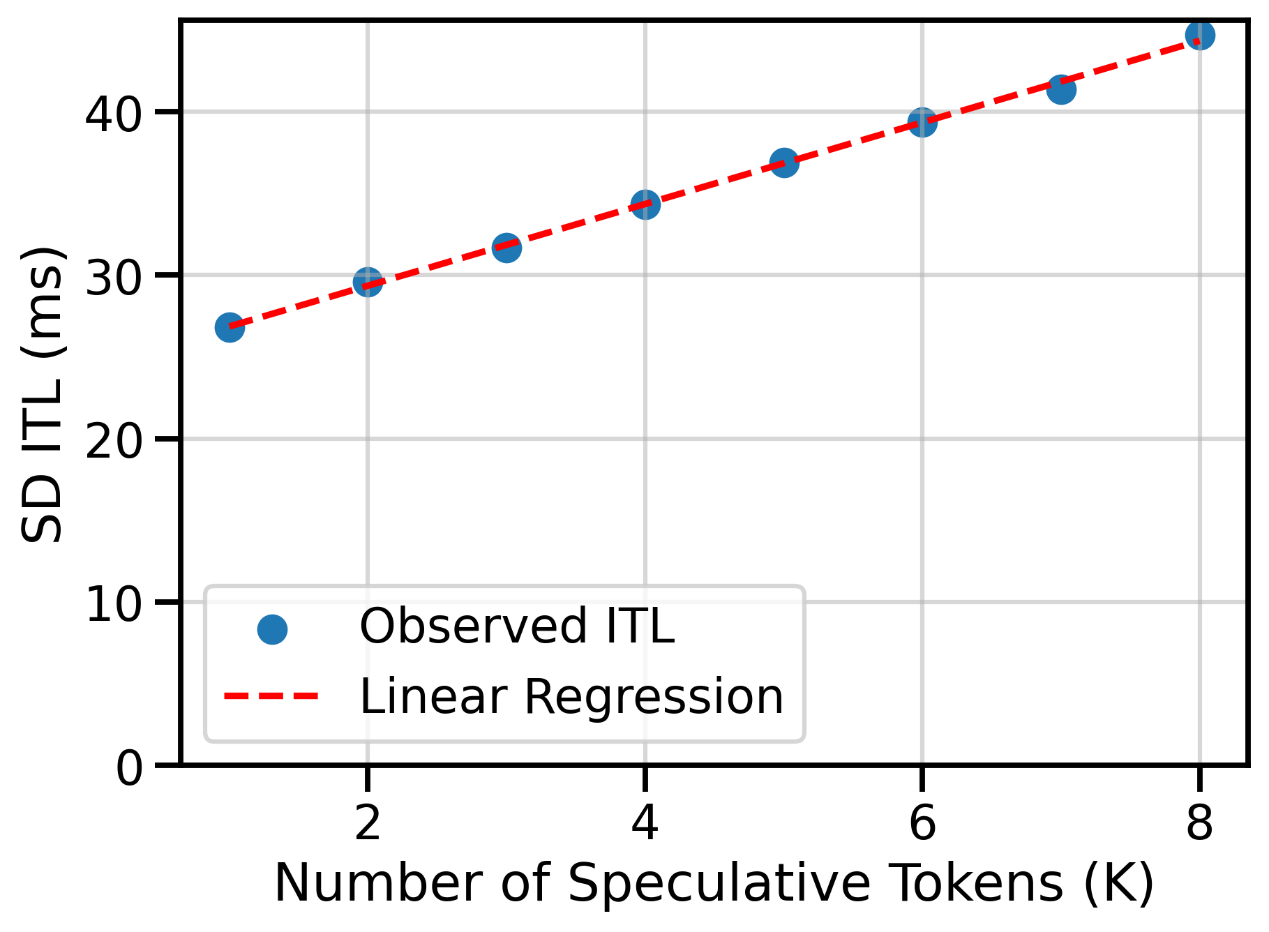
draft_model), run draft + target, and measure ITL while varying the number of speculative tokens (K). Because each additional speculative token triggers one extra draft forward pass, a linear fit of ITL vs K is a good approximation. The regression in Figure 1 can be interpreted as follows:- The Intercept: the target-model cost inside the SD loop
- The Slope: the incremental draft-model cost per additional speculative token
With those two measurements, we can compare per-token runtimes across graph modes in Table 1. “SD Runtime” comes from the ITL regression (Piecewise CG, inside SD), and “Standalone Runtime” is the median ITL from vllm bench serve without SD (Full CG). For this setup, the draft model is 9.10% faster under full graphs, while the target model is 2.91% faster.
| Model | SD Runtime (Piecewise CG) | Standalone Runtime (Full CG) | Runtime Reduction |
|---|---|---|---|
| Qwen3-1.7B | 2.50 ms | 2.27 ms | 9.10 % |
| Qwen3-32B | 24.36 ms | 23.65 ms | 2.91 % |
Forecasted End-to-end Impact
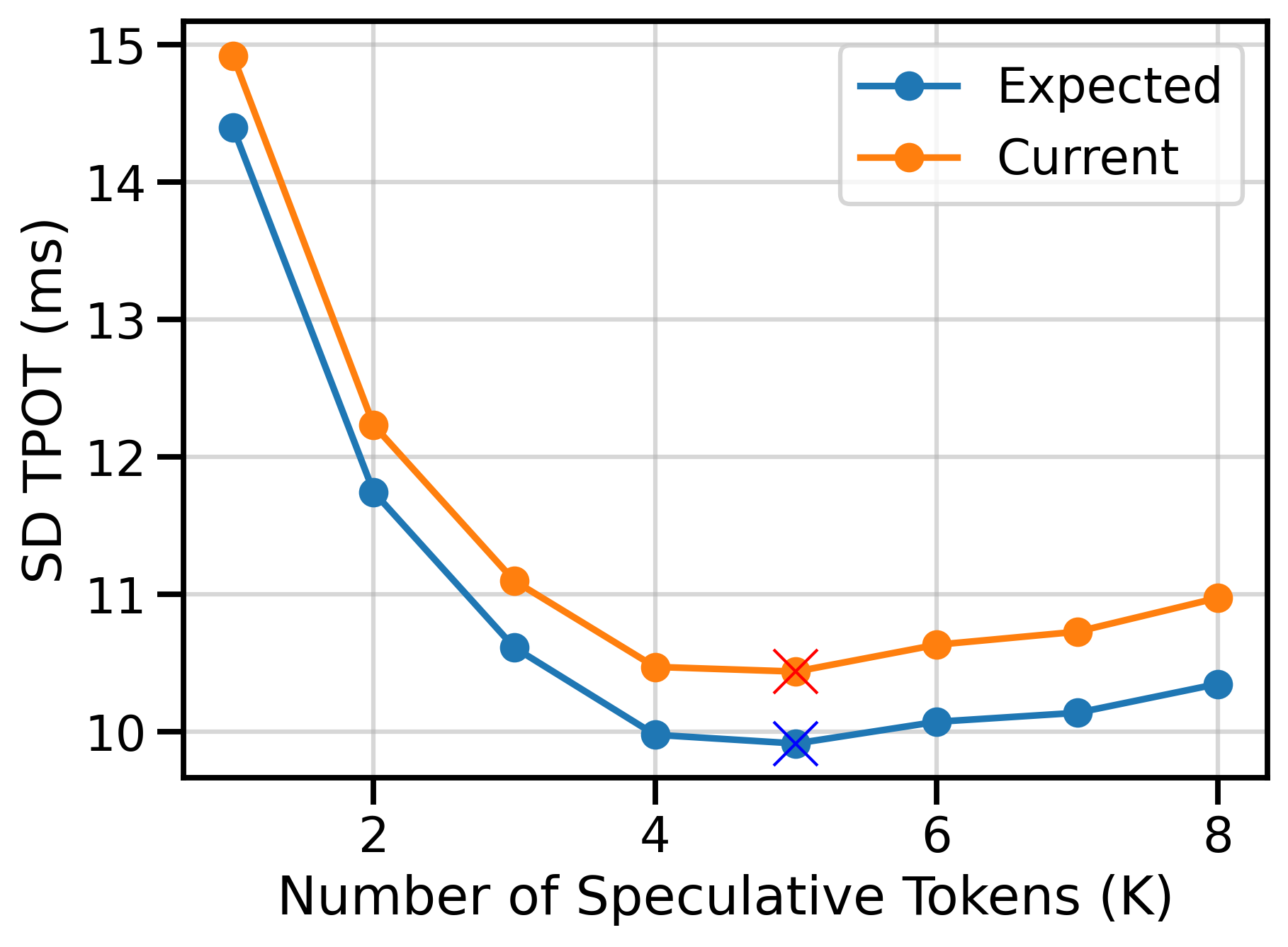
Assuming we could realize those per-token reductions inside speculative decoding, what does that translate to in terms of TPOT? I use the formula below to forecast the speedups for full CUDA graphs. \[ \text{TPOT} = \frac{\text{ITL}}{\text{AL}} = \frac{T_{d} \cdot K + T_{t}}{\text{AL}} \]
where \(T_{d}\) is the runtime of the draft model, \(T_{t}\) is the runtime of the target model, \(K\) is the number of speculative tokens, and \(\text{AL}\) is the acceptance length. Figure 2 shows the TPOT values under Piecewise CG (Current), and Full CG (Expected). The minimum (best) TPOT values for each curve are marked with a cross. At \(K=5\)1, the TPOT improves from 10.43ms to 9.91ms (4.9% improvement). The speedup ratios over vanilla decoding grow from 2.26× to 2.37× for Qwen3-32B (1.7B drafter) on MT-Bench.
Summary
Supporting Full CG for speculative decoding could improve speedup ratios by ~5% from 2.26× to 2.37× over vanilla decoding. When I started this analysis, I expected larger improvements (closer to 20%), but the target model dominates overall ITL, so draft-side gains translate to single-digit TPOT gains. Nevertheless, this improvement would positively impact the performance of draft_model across all workloads. The same method could be applied to estimate the performance gains for other combinations of draft, target models, and datasets.